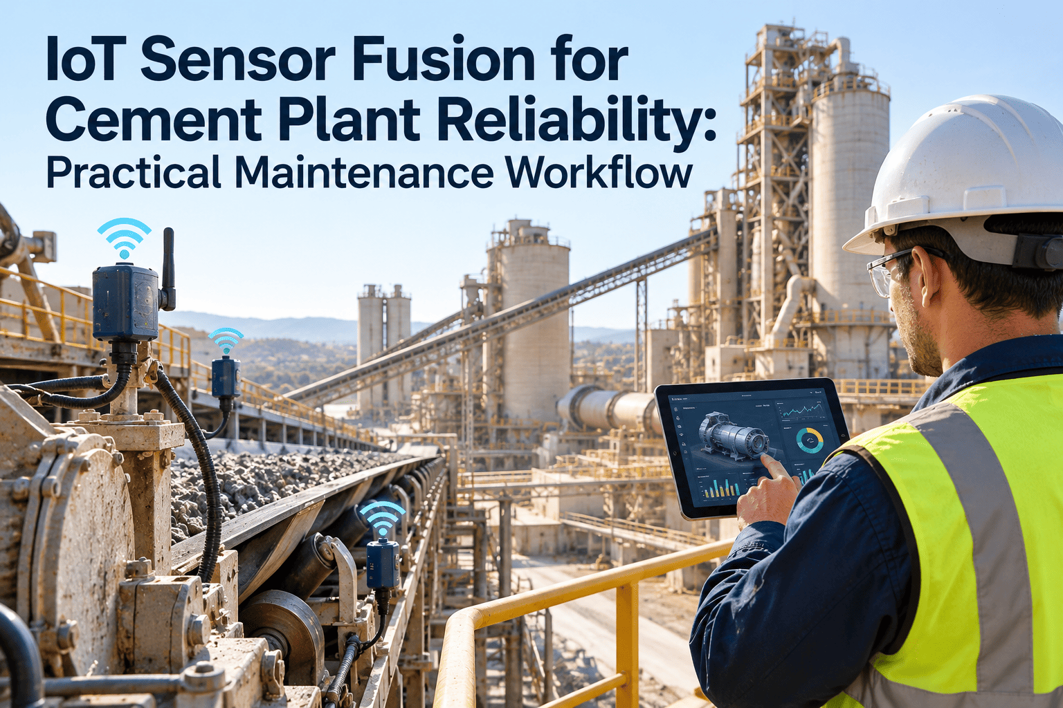
A cement plant kiln runs 8,000 hours a year, generating thousands of sensor readings every minute — bearing temperatures, vibration spectra, shell temperatures, inlet pressures, exhaust gas compositions, drive current signatures. Each of these readings, taken alone, tells a narrow story. A bearing temperature of 78°C is either normal or abnormal depending on ambient temperature, load, speed, and lubrication state. A DCS alarm set at 85°C catches failures after they have already begun. What catches failures weeks earlier — before the temperature moves at all — is the subtle correlation shift between bearing temperature, vibration amplitude, and drive current that emerges as a bearing starts to wear. No single threshold catches this. Multivariate sensor fusion AI does. Start an OxMaint free trial and see how multivariate anomaly scoring works on your plant's actual sensor data, or book a 30-minute demo with a cement industry AI specialist.
OxMaint AI · Cement Plant Anomaly Detection
Single-Parameter Alarms Miss 60% of Cement Equipment Failures.
Multivariate Sensor Fusion AI Catches What Thresholds Can't.
When vibration, temperature, pressure, and current shift subtly together — but none triggers an alarm alone — the failure is already developing. Only multivariate AI sees the pattern.
The Detection Gap
Why Single-Parameter Alarms Fail in Cement Plants
DCS threshold alarms are designed to respond to a parameter that has already crossed a limit. They are reactive by definition. The failure mode has been developing for days or weeks before the alarm fires — and the damage is already done.
Monitors each sensor independently against a fixed threshold
Alarm fires when a parameter exceeds a preset limit
No awareness of relationships between sensors
Detects failures only after physical degradation produces a parameter shift
Average warning lead time: 2–6 hours before failure
Misses failures that manifest only as correlation changes — no single parameter exceeds its limit until damage is severe
Catches approximately 40% of developing failures in time to prevent unplanned downtime
Models the normal correlation structure between all sensors simultaneously
Detects anomalies when the relationship pattern shifts — not individual values
Understands that 78°C bearing temperature is anomalous at certain vibration and load combinations, normal at others
Identifies developing failures 3–6 weeks before individual parameters exceed thresholds
Average warning lead time: 21–42 days before failure
Detects emergent failure signatures invisible to any individual sensor threshold
Catches approximately 95% of developing failures with sufficient lead time for planned intervention
How It Works
The Mechanics of Multivariate Anomaly Detection in Cement Equipment
Understanding what multivariate sensor fusion AI actually does — not in abstract terms, but in the specific context of cement plant equipment — makes the difference between deploying it effectively and treating it as a black box.
01
Baseline Learning: What Normal Looks Like
The AI model ingests 6–12 weeks of historical sensor data for each asset — across all operating conditions, loads, ambient temperatures, and production rates. It builds a multivariate model of normal: not just "bearing temperature is normally 70–78°C" but "bearing temperature is normally 70–74°C when vibration is 2.1 mm/s, speed is 1,480 RPM, and ambient temperature is 32°C." Each operating condition gets its own normal envelope.
Result: A dynamic baseline that adjusts to operating conditions in real time — eliminating false alarms that plague fixed-threshold systems.
02
Continuous Correlation Monitoring
During live operation, the AI monitors not just sensor values but the relationship matrix between all sensors simultaneously. A cement mill with 12 monitored parameters produces 66 pairwise correlation relationships. When bearing wear begins, the correlation between vibration amplitude and bearing temperature tightens before either variable moves far enough to trigger a threshold alarm. This is the signal the AI catches — invisible to any DCS alarm logic.
Result: Failure signatures detected at the earliest emergent stage — not at the point of obvious degradation.
03
Anomaly Scoring and Root Cause Attribution
When the model detects a correlation shift, it generates an anomaly score and identifies which sensors are driving the deviation — not just "something is wrong with the mill" but "the drive-end bearing shows early thermal-vibration coupling consistent with lubrication degradation, with 87% confidence." This attribution allows maintenance teams to take targeted action rather than running a full investigation.
Result: Specific, actionable alerts with root cause attribution — not generic equipment alarms that create more investigation work than they save.
04
Work Order Generation and CMMS Integration
When an anomaly score crosses a configured threshold, OxMaint automatically generates a maintenance work order — pre-populated with the asset details, anomaly description, sensor readings, and recommended inspection action. The work order is routed to the maintenance team's mobile app. The AI's detection is directly connected to the maintenance execution workflow without any manual handoff.
Result: Zero gap between AI detection and maintenance action. Every anomaly generates a traceable work order, creating an audit trail for reliability improvement.
Equipment Coverage
Where Multivariate Sensor Fusion Delivers the Highest Value in Cement Plants
Not all cement equipment benefits equally from multivariate analysis. These five asset classes have the highest failure cost, the clearest multivariate failure signatures, and the greatest detection lead time advantage over single-parameter alarms.
Rotary Kiln Drive System
$20K–$50K per hour downtime
Fused sensor inputs
Girth gear vibration
Shell temperature profile
Drive motor current
Kiln torque
Tire and roller contact
Failure signature: Early refractory hot spot develops as shell temperature anomaly correlates with torque fluctuation — weeks before shell scan shows visible damage. Lubrication breakdown appears as girth gear vibration-current correlation shift before noise is audible.
Detection lead time advantage: 18–35 days vs. 4–8 hours for single-parameter alarms
Vertical Roller Mill (VRM)
$500K–$1.2M repair cost per major failure
Fused sensor inputs
Roller bearing vibration (DE & NDE)
Grinding table power
Classifier speed
Differential pressure
Roller bearing temperature
Failure signature: Classifier motor bearing wear first appears as subtle correlation change between NDE bearing vibration and classifier speed — not a temperature rise. Power fluctuation becomes correlated with bearing vibration 3–4 weeks before audible bearing noise develops.
Detection lead time advantage: 21–42 days vs. 6–12 hours for single-parameter alarms
Preheater ID Fan
245 TPH kiln feed loss per fan trip
Fused sensor inputs
Fan bearing vibration (x, y, z)
Inlet static pressure
Motor current
Shaft speed
Bearing temperature (DE & NDE)
Failure signature: False temperature trip risk is detected as single-sensor divergence from the correlated thermal-vibration baseline — the AI flags a sensor drift event before operators respond to a false alarm with an unplanned shutdown. Real bearing failures show different multivariate patterns.
Detection lead time advantage: Prevents false trips and catches real failures 14–28 days earlier than threshold alarms
Cement Mill Ball Mill
$180K–$420K per unplanned stoppage
Fused sensor inputs
Mill body vibration
Trunnion bearing temperature
Drive pinion vibration
Mill motor power
Separator bearing temperature
Failure signature: Liner wear progression shows as gradual mill body vibration-power correlation shift over 4–6 weeks. Trunnion bearing degradation produces temperature-vibration coupling that develops 3 weeks before any individual measurement crosses its alarm limit.
Detection lead time advantage: 15–30 days vs. 2–8 hours for single-parameter alarms
Clinker Cooler Fans
Direct clinker quality and output impact
Fused sensor inputs
Fan bearing vibration
Outlet air temperature
Motor current draw
Damper position
Clinker temperature profile
Failure signature: Cooler grate plate wear appears as correlation shift between fan pressure output and clinker exit temperature — a multivariate signature that single sensors cannot generate independently. Blade erosion from clinker dust shows as current-vibration relationship drift weeks before performance drops measurably.
Detection lead time advantage: 14–25 days vs. 4–10 hours for single-parameter alarms
Your DCS Alarm System Is Watching the Symptoms.
OxMaint AI Watches the Pattern.
Multivariate anomaly detection on your existing sensor infrastructure — no new hardware, no threshold configuration, and detection lead times measured in weeks instead of hours.
Performance Data
What Multivariate AI Detection Delivers vs. Single-Parameter Baselines
The performance gap between single-parameter threshold alarms and multivariate AI detection is measurable across every dimension that matters operationally — lead time, false alarm rate, and total maintenance cost.
| Performance Metric |
Single-Parameter Alarms |
Multivariate Sensor Fusion AI |
Operational Impact |
| Average detection lead time |
2–8 hours before failure |
14–42 days before failure |
Shifts from emergency response to planned intervention |
| Failure detection coverage |
~40% of developing failures caught in time |
~95% of developing failures caught with lead time |
55% more failures prevented rather than responded to |
| False alarm rate |
High — fixed thresholds don't adjust to operating conditions |
Low — dynamic baselines account for load, ambient, and process variations |
Operators trust alerts and act on them; threshold alarm fatigue is eliminated |
| Root cause attribution |
None — parameter exceeded a limit; cause is unknown |
Specific sensor contribution weighting with failure mode classification |
Targeted inspection rather than full equipment teardown |
| Maintenance intervention cost |
Emergency repair rate: 3.4× planned cost |
Planned intervention rate: baseline cost |
Immediate ROI on first major failure averted |
| Sensor drift detection |
Not detected — single sensor drift is invisible to itself |
Detected as deviation from correlated sensor group |
Prevents false trips and corrupted condition monitoring baselines |
FAQs
Technical Questions from Cement Plant Reliability Engineers
Does OxMaint's multivariate AI require new sensors or hardware to be installed?
No. OxMaint connects to existing DCS, SCADA, and condition monitoring sensors via standard OPC-UA and historian interfaces. The multivariate models run on data the plant is already collecting — the AI layer adds analytical depth without requiring instrumentation changes. Most cement plants achieve full sensor fusion model activation within 4–6 weeks of data integration.
See the integration process in a free trial.
How long does the AI need to learn a normal baseline before it can generate reliable alerts?
The baseline learning period is typically 6–8 weeks of operational data — covering enough variation in load, ambient conditions, and production rate to build a robust multivariate normal model for each asset. During this period the system generates provisional alerts for review. Full production-confidence alerting begins at week 8–10. For assets with historical data in the CMMS, this period can be compressed significantly.
How does the system distinguish between a real failure signal and a normal process change that looks anomalous?
OxMaint's multivariate models account for known process changes — production rate shifts, raw material changes, ambient temperature variations — by conditioning the anomaly score on the operating context. When a plant increases feed rate, the AI adjusts the expected correlation structure accordingly rather than flagging the change as an anomaly. Operators can also annotate known process events, which train the model to recognize and exclude them from anomaly scoring.
Book a demo to see the model configuration interface.
What happens when a sensor fails or goes offline — does the model break down?
OxMaint's sensor fusion models are designed to be fault-tolerant. When a sensor drops out, the model continues operating on the remaining correlated sensors — reducing analytical precision slightly but maintaining detection capability on the surviving sensor group. The sensor outage itself is flagged as a data quality event requiring calibration attention, preventing the scenario where a failed sensor corrupts the AI's baseline silently.
How does OxMaint's multivariate AI connect to the maintenance workflow after detecting an anomaly?
Every anomaly score that exceeds the configured alert threshold automatically generates a work order in OxMaint's CMMS — pre-populated with the asset ID, anomaly description, contributing sensors, anomaly score history, and a recommended inspection action based on the failure mode classification. The work order routes to the assigned maintenance team's mobile app. There is no manual step between AI detection and maintenance response.
See the full detection-to-work-order workflow in a free trial.
OxMaint AI · Multivariate Anomaly Detection · Cement
The Failure Your Alarms Won't Catch Is Developing Right Now.
OxMaint's multivariate sensor fusion AI connects to your existing sensors and starts detecting correlation anomalies that DCS thresholds miss entirely — with detection lead times measured in weeks, not hours. Most cement plants are generating AI alerts within 10 weeks of data integration.