A biscuit manufacturer running three production lines faced the same problem every year: three weeks before the Christmas peak, a primary packaging line went down for unplanned repairs. The maintenance team had no visibility into the demand calendar. The production planner had no visibility into asset condition. Both were working from their own systems, with no connection between them. The emergency repair cost $94,000 in contractor fees, expedited parts, and lost production — all of it preventable if the PM had been scheduled eight weeks earlier during the summer trough. AI-powered demand forecasting has transformed how FMCG plants plan production. The same data that tells you when your lines will run at 100% capacity for 14 straight weeks should be telling your maintenance scheduler when to take equipment down for overhaul, bearing replacement, and calibration. It almost never does — because the two systems don't talk. Plants that integrate demand forecasting with maintenance scheduling reduce peak-season breakdowns by 60–75%, cut emergency maintenance costs by $80,000–$200,000 per year, and achieve 15–22% higher OEE during high-demand periods. Start your free trial or book a demo to see demand-aligned maintenance scheduling in action.
60–75%
reduction in peak-season breakdowns when maintenance windows align with demand troughs
$80K–$200K
annual emergency maintenance cost savings from proactive demand-driven scheduling
15–22%
higher OEE during peak production periods when assets are serviced ahead of demand spikes
8–12 wks
average advance window available in AI demand forecasts — enough time for full planned overhauls
Oxmaint — Supply Chain Integration & Capacity Planning
Stop Scheduling Maintenance in a Demand Vacuum. Connect the Two Systems.
Oxmaint integrates with your demand forecasting and production planning data to automatically flag maintenance windows during low-demand periods — so every overhaul, PM, and inspection happens when the line can afford to be down, not when a breakdown forces it.
Why Maintenance Scheduling and Demand Forecasting Operate in Separate Silos
In most FMCG plants, the maintenance team and the production planning team have fundamentally different information systems, different reporting lines, and different success metrics. The maintenance manager measures PM compliance rate, MTBF, and cost per work order. The production planner measures line utilisation, fill rate, and schedule adherence. Both are optimising for their own KPIs — and neither has visibility into the constraints of the other. The result is predictable: maintenance gets scheduled based on calendar intervals and technician availability. Demand peaks get scheduled based on customer orders and inventory targets. The two schedules collide during peak season, every year, producing exactly the emergency that everyone knew was coming but nobody prevented.
How Most FMCG Plants Schedule Maintenance
✗Fixed calendar intervals — every 90 days regardless of production load
✗Technician availability drives timing — not demand calendar
✗No visibility into upcoming demand spikes when scheduling PMs
✗Emergency repairs accepted as normal during peak season
✗Post-peak catch-up maintenance creates a second bottleneck
✗Demand forecasts sit in ERP — maintenance team never sees them
How Demand-Integrated Plants Schedule Maintenance
✓Maintenance windows pulled from 8–12 week demand forecast troughs
✓PM intervals flex with asset condition and production load data
✓Every overhaul planned during low-demand periods — never peak season
✓Emergency repairs near zero during peak — assets serviced in advance
✓Demand forecast feeds CMMS scheduling automatically
✓Maintenance and production plans reviewed together in one system
The Real Cost of Peak-Season Maintenance Failures
When a packaging line fails during peak demand season, the financial impact is not just the repair cost — it is the cascading effect across the entire supply chain. A line running at $32,000 per hour in throughput value loses that revenue every hour it sits idle. Emergency contractors charge 2.5–4x normal labour rates. Expedited parts shipments cost 3–8x standard freight. Customer service levels drop, retailer penalties trigger, and the premium production window narrows. The maintenance team that could have addressed the failing bearing eight weeks ago for $4,000 now faces a $140,000 event. Every FMCG plant has experienced this. Few have built the system that prevents it.
Peak-Season Breakdown: True Cost Breakdown
Typical FMCG packaging line failure during a 6-week peak demand window
Lost Throughput
Line down 18–36 hours × $22K–$38K/hr throughput value — revenue permanently lost, not recovered
$40K–$135K
Emergency Repair Labour
Emergency contractor rates 2.5–4x standard — weekend and overnight call-out premiums included
$12K–$28K
Expedited Parts & Freight
Air freight + premium supplier sourcing for parts that would cost 3–8x less ordered in advance
$4K–$18K
Retailer Penalties & Chargebacks
Short shipments and late deliveries trigger contractual penalties — particularly severe in UK grocery retail
$8K–$35K
Planned Maintenance Cost (Avoided)
Same repair scheduled 8 weeks earlier during demand trough — standard labour, stocked parts, planned shutdown
$3K–$8K
Emergency vs. Planned Cost Ratio
15–30× More Expensive
The repair itself is rarely the largest cost. Lost throughput and retailer penalties typically account for 70–80% of the total event cost. Oxmaint's demand-integrated scheduling prevents this by surfacing every maintenance window 8–12 weeks ahead of demand peaks — when the line can be taken down with zero throughput impact.
How AI Demand Forecasting Creates Maintenance Windows
Modern AI demand forecasting models — whether built on gradient boosting, LSTM neural networks, or ensemble methods — produce rolling 12–26 week demand projections with confidence intervals by SKU, by line, and by plant. These forecasts are not just production targets. They contain embedded maintenance windows: the 4-day trough between promotional periods, the 11-day gap before a seasonal ramp, the 3-week shoulder between summer and autumn trading. Maintenance schedulers almost never see this data. It sits in the ERP or the demand planning system, visible to the supply chain team but invisible to the CMMS. Connecting these two data streams is the core of demand-integrated maintenance — and it requires no new forecasting capability, just routing the existing data to the right place.
Rolling Demand Forecast
8–26 Week Horizon
AI forecasts project demand by line and SKU across 8–26 weeks. Troughs in this data are maintenance windows — periods where planned downtime has zero or minimal throughput impact. Most CMMS systems never receive this data.
Seasonal Pattern Recognition
Annual Cycle Mapping
AI models identify recurring seasonal demand patterns — Easter ramps, summer troughs, Christmas peaks, January resets. These patterns repeat each year, making next year's maintenance windows predictable 12+ months ahead.
Maintenance Window Scoring
Automated Prioritisation
Each potential maintenance window is scored by duration (hours available), demand impact (throughput at risk), and asset urgency (condition data). The CMMS surfaces the highest-value windows first — maximising PM completion before peak demand arrives.
Cross-Line Conflict Detection
Schedule Optimisation
When multiple assets need maintenance in the same window, AI resolves conflicts by asset criticality and demand risk. It prevents the scenario where three lines are down simultaneously during a period that looked low-demand on a single-line view.
Demand Volatility Buffering
Risk Management
AI forecasts include confidence intervals. High-volatility demand periods — new product launches, promotional events, weather-sensitive categories — get a maintenance exclusion buffer, protecting scheduled downtime from being overridden by demand surges.
Forecast-to-Actual Variance Tracking
Continuous Learning
When actual demand deviates from forecast, the system updates future maintenance window recommendations. Over time, the model learns which forecast signals are reliable for scheduling and which require a larger buffer — improving window quality each cycle.
Demand Integration — Oxmaint
Your Demand Forecast Already Contains Next Year's Maintenance Windows.
Oxmaint connects to your ERP or demand planning system to surface maintenance windows automatically — ranked by duration, demand impact, and asset urgency. Your maintenance scheduler sees the right window at the right time, every time.
The Three-Layer Model: Connecting Demand, Assets, and Maintenance
Demand-integrated maintenance scheduling operates across three data layers that must communicate in real time. Layer one is the demand signal — the AI forecast with confidence intervals, updated weekly. Layer two is the asset condition layer — the CMMS data showing PM due dates, condition trends, failure risk scores, and maintenance backlog by asset. Layer three is the scheduling layer — the optimisation engine that matches maintenance need against demand opportunity, producing a rolling 12-week maintenance calendar that is never in conflict with the production plan. Most FMCG plants have all three layers. They just have no integration between them.
1
Layer 1: Demand Signal — The Opportunity Calendar
Source: AI demand forecast from ERP (SAP, Oracle, Blue Yonder, o9, Anaplan). Updated weekly. Key data: projected demand by line, confidence interval width, promotional events calendar, seasonal ramp dates, and committed customer orders. Any period where forecast demand falls below 75% of peak capacity for 48+ consecutive hours is a candidate maintenance window.
Weekly Update
2
Layer 2: Asset Condition — The Urgency Register
Source: CMMS (Oxmaint). Key data: PM due dates with overdue risk score, condition trend deviation from commissioning baseline, maintenance cost ratio by asset, MTBF trajectory, and failure probability in next 90 days. Assets are ranked by urgency: Red (overdue or high failure risk), Amber (due within 30 days), Green (healthy, monitor). Red and Amber assets get priority assignment to the next available demand window.
Daily Update
3
Layer 3: Scheduling Engine — The Integration Output
The scheduling engine matches Layer 2 urgency against Layer 1 opportunity, constrained by technician availability, spare parts lead times, and regulatory requirements (BRC, SQF). Output: a rolling 12-week maintenance calendar, updated weekly, showing every planned PM and overhaul in a demand trough — with a live conflict alert if production planning attempts to schedule production into a confirmed maintenance window.
Real-Time
Seasonal Demand Patterns: Where the Maintenance Windows Hide
FMCG demand follows predictable seasonal rhythms. Every category has its own pattern, and AI forecasting models learn these patterns from 3–5 years of historical data. The patterns that create production peaks also create maintenance troughs — and those troughs are the most valuable asset your maintenance scheduler has. Understanding the demand calendar of your specific category is the first step toward a maintenance schedule that is never in conflict with customer demand.
Confectionery & Snacks
Peak: Oct–Dec (Halloween, Christmas), Feb (Valentine's). Troughs: Jan reset (2–3 weeks), May–June (pre-summer). Maintenance windows: January is the single most valuable maintenance month — demand drops 40–60% from December peak. Full overhauls, line changeovers, and bearing replacements should concentrate here every year without exception.
Primary window: January · Secondary: May–June
Beverages & Soft Drinks
Peak: May–August (summer), Dec (festive). Troughs: Oct–Nov (pre-Christmas buildup is moderate), Jan–Feb (deepest trough). Maintenance windows: October–November offers 6–8 weeks before Christmas ramp — ideal for filler overhauls and CIP system servicing. January provides a secondary deep trough.
Primary window: Oct–Nov · Secondary: January
Personal Care & Household
More stable year-round demand with moderate seasonal variation. Promotional events (retailer campaigns, Black Friday) create short peaks. Troughs: Late January, mid-August. Maintenance windows: August offers 3–4 consistent low-demand weeks across most personal care subcategories — the most reliable annual maintenance window in this category.
Primary window: August · Secondary: Late January
Building the Demand-Maintenance Integration: Step by Step
Integrating AI demand forecasting with maintenance scheduling does not require replacing your ERP, your CMMS, or your forecasting model. It requires connecting the outputs of systems you already own — routing the demand forecast into the maintenance scheduling workflow so that every PM, overhaul, and inspection is placed in a window where the production plan can accommodate it. The implementation follows four phases, each with a specific output that builds on the previous one.
Phase 1
Forecast Data Access
Extract 12-week rolling demand forecast from ERP by line and SKU
Map forecast output to production line assignments in CMMS
Define maintenance window threshold: % capacity below which downtime is acceptable
Set confidence interval filter — exclude windows with high forecast uncertainty
Output: Demand calendar visible in CMMS
Phase 2
Asset Urgency Scoring
Score every asset by maintenance urgency: PM overdue risk, condition deviation, cost ratio
Calculate failure probability score for next 12 weeks per asset
Classify assets: Red (must service before next peak), Amber (service in next trough), Green
Estimate work duration for each Red and Amber asset — hours required for each job
Output: Prioritised maintenance backlog with time estimates
Phase 3
Window Matching
Match Red and Amber assets to available demand windows by line and duration
Check technician and parts availability against each window candidate
Resolve cross-line conflicts — no more than one critical line down per window
Generate draft 12-week maintenance schedule aligned to demand trough calendar
Output: Demand-aligned 12-week maintenance plan
Phase 4
Live Integration
Weekly forecast refresh updates available maintenance windows automatically
Conflict alerts fire when production planning overwrites a confirmed maintenance window
KPI dashboard tracks: windows used, windows missed, peak-season emergency rate
Monthly review: compare planned vs actual — tighten threshold calibration each cycle
Output: Self-updating demand-maintenance calendar
Measuring the Impact: KPIs That Prove Demand-Integrated Maintenance Works
The financial case for demand-integrated maintenance is measured across four KPI dimensions. Each can be tracked from data that already exists in your CMMS and ERP — no new sensors, no new reporting infrastructure. The first measurement cycle typically shows impact within 90 days of integration, with full annual value visible by the end of the first peak season post-implementation.
Before Demand Integration
Peak-season emergency maintenance rate: 4–8 events per peak period
Emergency maintenance as % of total maintenance spend: 28–40%
OEE during peak: 68–74% (breakdown losses dominate)
Maintenance windows utilised from demand forecast: 0% (no visibility)
Average lead time for planned maintenance: 3–5 days (reactive)
Annual retailer penalties from supply failures: $40K–$120K
After Demand Integration
Peak-season emergency maintenance rate: 1–2 events per peak period
Emergency maintenance as % of total maintenance spend: 8–14%
OEE during peak: 83–89% (planned availability replaces breakdown losses)
Maintenance windows utilised from demand forecast: 85–95%
Average lead time for planned maintenance: 4–8 weeks (proactive)
Annual retailer penalties from supply failures: $5K–$18K
The Annual ROI of Demand-Integrated Maintenance Scheduling
The value of connecting demand forecasting to maintenance scheduling compounds across multiple cost categories simultaneously. Reduced emergency events lower direct repair costs. Higher peak OEE increases throughput revenue. Lower retailer penalties protect gross margin. Reduced unplanned downtime improves workforce efficiency. For a mid-size FMCG plant running two to four production lines, the combined annual value typically reaches $350,000–$620,000 — against an integration and platform investment measured in thousands, not hundreds of thousands.
Annual ROI: Demand-Integrated Maintenance Scheduling
Mid-size FMCG plant · 3 production lines · 2 major demand peaks per year · 14-person maintenance team
Emergency Repair Avoidance
Reduction from 6–10 to 1–2 peak-season emergency events × $45K–$140K average event cost
$220,000
Peak OEE Improvement
8–14% OEE gain during 12 weeks of peak demand × $22K–$38K/hr throughput value × reduced downtime hours
$145,000
Retailer Penalty Reduction
Fewer short shipments and late deliveries during peak — contractual penalty exposure reduced 70–85%
$68,000
Planned vs Emergency Labour Differential
Shifting 6+ emergency events to planned work at standard rates — 2.5–4x labour cost premium eliminated
$42,000
Parts Cost Normalisation
Replacing expedited air freight + premium sourcing with standard stocked parts ordered in advance
$24,000
Oxmaint + Integration Investment
Platform licence + ERP integration setup + onboarding — full demand-maintenance scheduling capability
$18K–$28K/yr
Net Annual Value — Demand-Integrated Maintenance
$499K+ · 18–28× ROI
The largest single value driver is peak OEE improvement — converting unplanned breakdown hours into planned production hours during the periods when each production hour is worth the most. A single additional production hour during Christmas peak at a biscuit plant is worth more than 6 hours in January.
How Demand-Integrated Scheduling Changes CapEx and Budget Conversations
When maintenance managers can show that every major PM and overhaul is scheduled in a demand trough — with data linking the maintenance calendar to the production forecast — the budget conversation changes. Instead of defending reactive spend after the fact, the maintenance team presents a proactive investment plan: these assets will need service before the October peak, these are the windows available, this is the cost at planned rates versus the cost at emergency rates if deferred. The CFO who rejected the maintenance budget last quarter approves it when they see the emergency cost comparison.
Element
Before Integration
After Integration
Timing Justification
"The PM is overdue"
Scheduled 9 weeks before Oct peak — only window available
Cost if Deferred
Unknown — no forecast visibility
$140K emergency event modelled from last year's data
Production Impact
"We'll try to minimise downtime"
Zero throughput impact — demand trough confirmed in forecast
Budget Request
Reactive — emergency PO after failure
Planned — approved 8 weeks in advance at standard rates
CFO Response
Approve under duress — questions why not planned
Approves immediately — cost avoidance is self-evident
Labour Rate Applied
2.5–4× emergency premium
Standard planned rate — 60–75% less expensive
Demand integration does not change what maintenance needs to be done — it changes when and why. The same bearing replacement costs $4,200 planned and $18,500 emergency. The data that justifies the planned investment already exists in your ERP. Oxmaint surfaces it in the maintenance scheduling workflow automatically.
Frequently Asked Questions
Do we need to replace our ERP or demand planning system to integrate with Oxmaint?
No. Oxmaint integrates with existing demand planning systems via standard data export or API connection. The most common integration path is a weekly CSV or API feed of the rolling demand forecast by production line — a file your demand planning or supply chain team can set up in under a day. Oxmaint supports direct integration with SAP IBP, Oracle Demand Management, Blue Yonder, o9 Solutions, Anaplan, and most ERP demand modules. If your system produces a demand forecast, Oxmaint can consume it and surface maintenance windows from it.
What if our demand forecast is unreliable — will the maintenance windows also be unreliable?
Forecast quality is managed through confidence interval filtering. Oxmaint only surfaces maintenance windows from forecast periods with high confidence — typically where the forecast error (MAPE) is below 15–20%. Volatile forecast periods are automatically excluded from window recommendations and flagged as high-risk. Additionally, a demand buffer is applied: windows are only opened when forecast demand falls below 70–75% of peak capacity, not just below average. This means even a forecast that is off by 10–15% still leaves a valid maintenance window. Seasonal troughs in most FMCG categories are predictable enough that even lower-accuracy forecasting models identify them reliably.
How far in advance can we realistically plan maintenance using demand forecasting data?
Most FMCG demand forecasting systems produce reliable 8–12 week rolling forecasts, with 16–26 week seasonal plans available for annual peak planning. The 8–12 week window is sufficient to plan and execute all standard PMs, bearing replacements, seal overhauls, and most major component replacements — the procurement lead time for the majority of FMCG maintenance parts is 2–6 weeks. For complex overhauls requiring specialist contractors or long-lead parts, the 16–26 week seasonal forecast provides adequate lead time. The annual seasonal pattern recognition in AI models effectively gives you a 12-month maintenance planning horizon for any demand-pattern-based scheduling.
What happens when production planning overwrites a confirmed maintenance window?
Oxmaint generates a conflict alert when a production schedule change closes a confirmed maintenance window. The alert shows the specific assets affected, their current urgency score, the next available window (with its distance from the next demand peak), and the estimated risk cost if the PM is deferred past the peak. This is not an automated block — production always has override authority. But the maintenance manager now has quantified data to escalate: "if we close this window, these three assets go into peak season without service, and last year's data shows a 68% probability of an emergency event costing $85,000–$140,000." That conversation produces a different outcome than "we need to do the PM."
How do we handle maintenance for assets that serve multiple production lines with different demand patterns?
Shared assets — utilities, compressed air systems, CIP skids, conveyor infrastructure — are mapped to all lines they serve. The maintenance window for a shared asset is only valid when all lines it serves are simultaneously in a demand trough. Oxmaint calculates a composite demand score across all mapped lines and only surfaces a window when the combined demand falls below the maintenance threshold. For assets serving lines with very different demand patterns, Oxmaint identifies the best available window (minimum demand impact) and presents the estimated throughput risk alongside the urgency score — so the maintenance manager can make an informed trade-off rather than an uninformed one.
Oxmaint Supply Chain Integration
Your Demand Forecast Already Contains Next Year's Maintenance Windows. Start Using Them.
Every trough in your demand calendar is a maintenance opportunity. Every peak is a risk your current schedule may not be protecting. Connect the two — and stop discovering $140,000 emergencies the week before Christmas.
60–75%
fewer peak-season breakdowns
Get started in 3 steps
1Connect your demand forecast
CSV or API feed from your ERP — set up in under a day
2Score your asset urgency register
Red, Amber, Green ranking across every production asset
3Generate your demand-aligned schedule
12-week maintenance plan in your first week