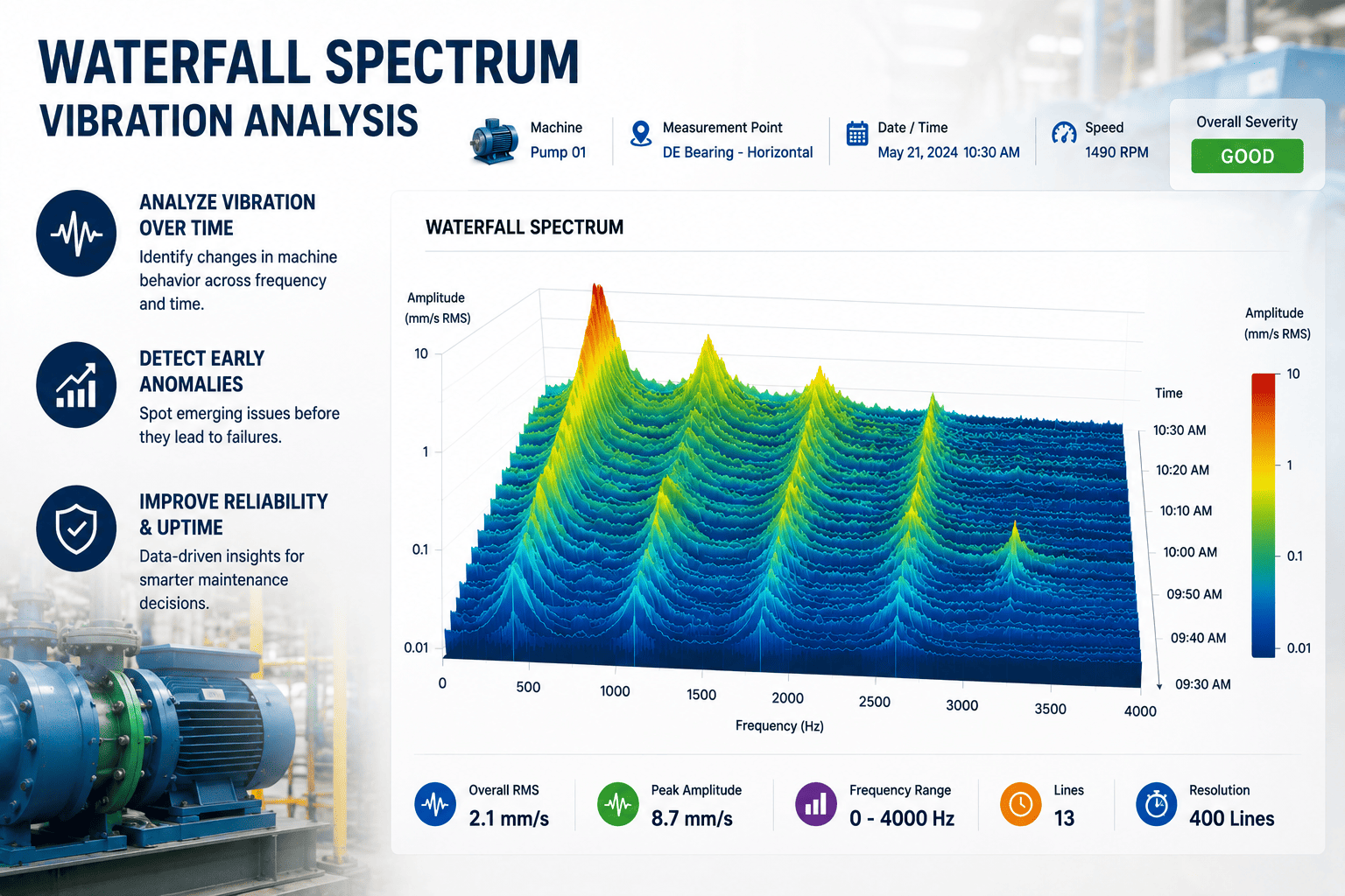
Vibration signatures hide the earliest whispers of machine failure — a bearing's inner race defect, a coupling's angular misalignment, or a structural resonance can surface in the frequency domain weeks before amplitude triggers a maintenance alarm. Waterfall and spectrum analysis convert raw accelerometer waveforms into trendable, time-stamped frequency plots that turn single-point RMS readings into predictive intelligence. For a 180-asset plant spending $42K annually on reactive repairs, a properly tuned waterfall program typically returns 4–6× its first-year cost by catching faults in the operator-visible window. Ready to put your FFT data to work? Start Free Trial and deploy a CMMS-linked vibration pipeline this quarter.
What if you could read a bearing defect three weeks before it fails?
Waterfall spectrum plots layer hundreds of FFT snapshots into a single time-mapped canvas — exposing fault-frequency drift, harmonic growth, and resonance creep that point readings miss. This guide unpacks the chart-reading workflow that reliability engineers use to move from alarm-driven maintenance to condition-driven intervention.
How a waterfall plot encodes time into frequency
A spectrum analysis takes a single time-domain waveform and decomposes it into its frequency components — amplitude on the Y-axis, frequency on the X-axis. A waterfall plot stacks successive spectra along a third axis (time or RPM), so every horizontal "ridge" in the 3D surface traces how a single frequency changed over hours, days, or production runs.
Mount & collect tri-axial data
Stud-mounted accelerometer on the bearing housing, 3–5 kHz Fmax for rolling-element bearings. ISO 10816 velocity thresholds (2.3–7.1 mm/s RMS for Class II machines) gate severity, but they don't tell you which fault — only the spectrum does.
Window, FFT, average
Apply a Hann window, 1,600–3,200 lines of resolution, 8–12 averages to suppress random noise. Each snapshot becomes one "slice" — a frequency vector with amplitude peaks at running speed (1×), harmonics, bearing defect frequencies, and line-frequency components.
Stack slices into the waterfall
Lay slices top-to-bottom along a time axis. Each peak becomes a ridge; a fault growing over weeks forms a ridge that brightens and rises. Trend the amplitude of that ridge and you've converted a point reading into a failure-forecast curve.
Trend ridge amplitude to alarm
Set a yellow alarm at 0.15 mm/s RMS on the BPFO ridge, red at 0.45 mm/s. At 3× baseline slope, raise a CMMS work order with 2–3 weeks of lead time — enough to schedule downtime, order the replacement bearing, and avoid a catastrophic secondary failure.
Bearing defect vs. imbalance vs. misalignment — the frequency fingerprint
Each mechanical fault has a characteristic frequency signature. Knowing the fingerprint lets you triage in seconds — before you ever leave the analysis screen — and prevents the expensive mistake of balancing a machine that actually needs realignment.
Non-integer defect frequencies calculated from bearing geometry. First sign: a low-amplitude peak (often <0.1 mm/s) at the BPFO with 1× sidebands. As the spall grows, harmonics appear and the ridge rises 3–10× over 2–6 weeks.
A single dominant peak at 1× shaft frequency. Radial vibration on both horizontal and vertical probes, phase difference ~90°. Amplitude tracks shaft speed linearly — confirm with a startup or coast-down run.
Angular or parallel misalignment between coupling halves produces a strong 2× peak, often with a smaller 1× component. Axial vibration is significant — a 50/50 radial/axial split is a hallmark. Phase across the coupling differs by ~180°.
A structural natural frequency excited by a passing shaft harmonic. The peak frequency does NOT change with RPM — it's locked to the structure. Confirm with a bump test or a run-up sweep; amplitude spikes sharply when 1× or 2× crosses the natural freq.
A 180-asset plant, $42K/yr in reactive bearing repairs
Consider a food-processing plant running 180 motors, pumps, and fans. Annual bearing failures averaged 23, costing $42,000 in emergency labor, expedited parts, and lost production. After deploying route-based vibration collection on a 30-day cycle with waterfall trending in their CMMS, the failure count dropped to 6 in year one.
Alarm-driven, point RMS readings
- 23 unplanned bearing failures per year
- $42K reactive spend (parts + OT labor + scrap)
- Avg. 11 hours downtime per failure event
- No trend history — failures arrived "without warning"
Waterfall-trended, CMMS-linked
- 6 unplanned failures in year one (74% reduction)
- $11K reactive spend — $31K redirected to planned work
- Avg. lead time from first detection to alarm: 21 days
- Every asset carries a 12-month spectral history in the CMMS
Program cost includes 2 route-based collectors, 18 stud-mounted sensors, and CMMS integration — recovered in under 11 weeks.
From first spectral signature to functional failure
The P-F curve maps the interval between a detectable fault signature (P) and functional failure (F). Spectrum analysis extends the P-F window dramatically — here's how each fault type progresses and how much lead time each gives you.
| Fault type | First spectral signature | P-F window | Failure mode if uncaught |
|---|---|---|---|
| Bearing outer-race defect | BPFO peak with 1× sidebands, <0.15 mm/s | 3–8 weeks | Spall propagates to cage fracture → sudden seizure |
| Bearing inner-race defect | BPFI with 1× sidebands, modulated amplitude | 2–6 weeks | Race fragmentation, secondary shaft damage |
| Rolling-element defect | BSF peak with FTF sidebands | 4–10 weeks | Element fracture, debris contamination of lubricant |
| Imbalance | 1× peak rising above ISO 10816 alarm | Weeks to months | Seal wear, bearing overload, fatigue cracking |
| Resonance | Fixed-frequency column brightens during run-up | Indefinite (if avoided) | Fatigue failure of structure or housing at stress concentration |
Closing the loop from spectrum to work order
A waterfall plot sitting in a standalone analyzer is an artifact. The same plot, attached to an asset record in your CMMS with automated alarm thresholds and a work-order trigger, becomes a maintenance decision. Here's what a properly integrated pipeline does at each stage.
Collect
Route-based or wireless sensors push tri-axial waveforms to the CMMS on a 7–30 day cycle, tagged with asset ID, RPM, and load.
Analyze
The CMMS runs FFT processing, identifies fault-frequency peaks against the asset's bearing geometry library, and appends a slice to the waterfall.
Trend
Ridge amplitudes for BPFO, BPFI, BSF, 1×, 2× are stored as time-series. Slope-based alarms fire when growth exceeds 3× baseline over 4 readings.
Act
A pre-filled work order opens with fault type, severity, recommended fix, and the spectral evidence attached — ready for scheduling.
Turn your FFT data into work orders this quarter
OxMaint ships with bearing-frequency libraries, ISO 10816 alarm templates, and a waterfall trending module that writes directly to your asset records. Deploy in days, not quarters.
Waterfall & spectrum analysis, answered
What's the difference between a spectrum plot and a waterfall plot?
A spectrum plot is a single FFT — frequency on X, amplitude on Y, captured at one moment. A waterfall plot stacks many spectra along a time (or RPM) axis so you can see how each frequency component evolves. The spectrum tells you what's wrong today; the waterfall tells you how fast it's getting worse and when it will cross your alarm threshold.
How often should I collect vibration data for waterfall trending?
For critical assets (ISO 10816 Class III+), collect every 7–14 days. For general plant equipment, a 30-day route is sufficient. The key is consistency — the waterfall's predictive power comes from ridge slope, and slope needs evenly spaced samples. Wireless continuous-monitoring sensors push a slice hourly and compress to daily trends, which is ideal for variable-speed or high-criticality machines. You can pilot this with a Start Free Trial on up to 25 assets.
Can I detect bearing defects without knowing the bearing part number?
Partially. You'll see a non-synchronous peak with 1× sidebands, which strongly suggests a bearing defect — but without the geometry you can't confirm which race or element is failing. Always capture bearing part numbers at install and load the defect frequencies (BPFO, BPFI, BSF, FTF) into the CMMS asset record so the spectrum annotator can label peaks automatically.
What Fmax and resolution should I use for rolling-element bearings?
Set Fmax to 3–5 kHz for machines under 3,600 RPM — bearing defect frequencies and their harmonics live in this band. Use 1,600–3,200 lines of resolution so closely spaced sidebands separate cleanly. For gearboxes or high-speed spindles, push Fmax to 10 kHz and add envelope (demodulated) spectrum to catch early-stage impacts that raw FFT misses.
How does OxMaint integrate waterfall trending with my existing CMMS?
OxMaint stores every spectrum slice against the asset record, auto-annotates bearing fault frequencies from a built-in geometry library, and triggers work orders when ridge slope crosses configurable thresholds (typically 3× baseline over 4 readings). The waterfall renders inline on the asset page alongside work-order history, so a reliability engineer can see the spectral evidence and the maintenance response in one scroll. To see it mapped to your asset hierarchy, Book a Demo with our team.
Stop reacting to alarms. Start reading the spectrum.
Deploy waterfall trending, bearing-frequency auto-annotation, and CMMS-linked work orders in days. Your first 25 assets are free for 14 days.
Free 14-day trial · No credit card