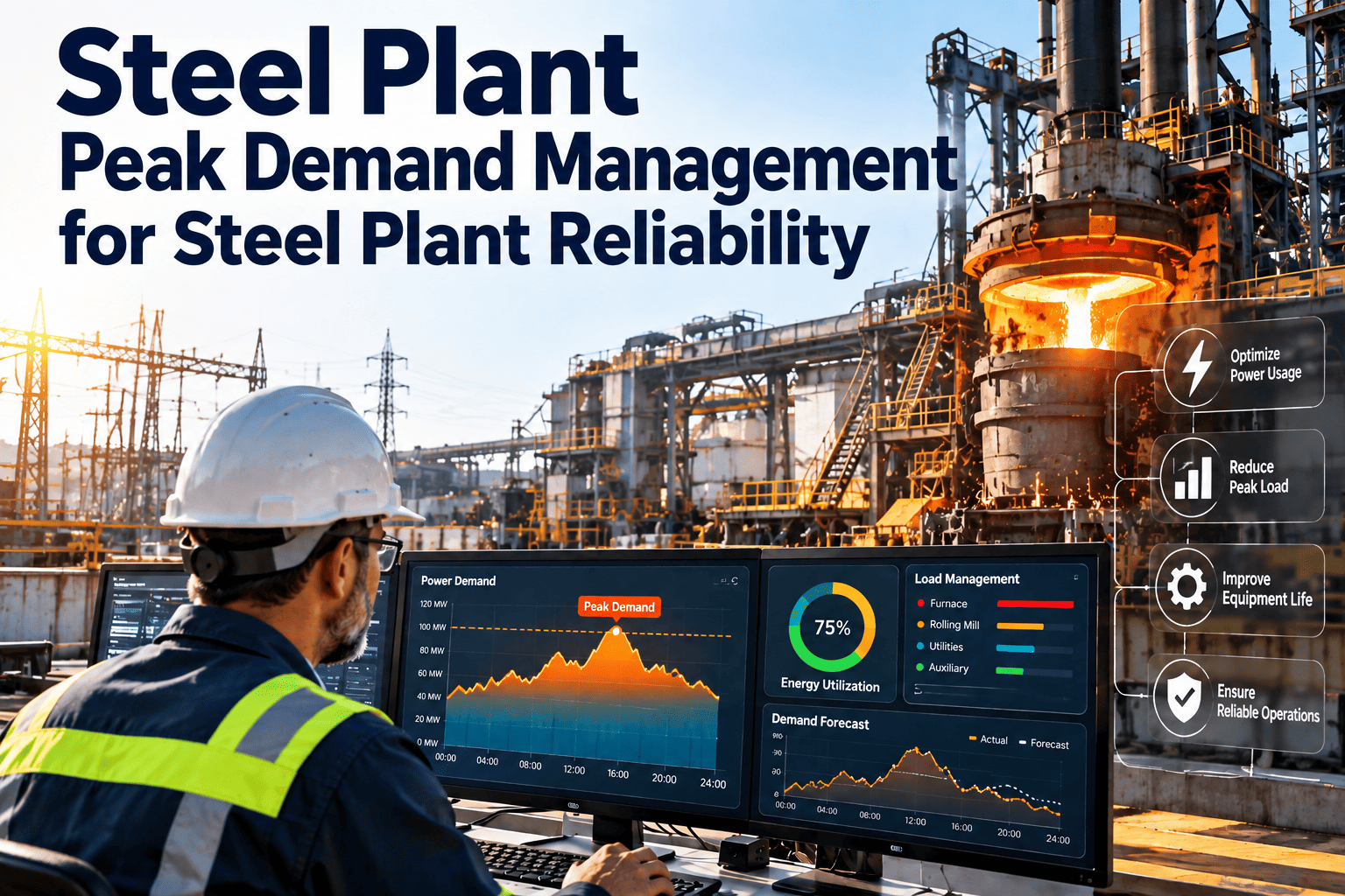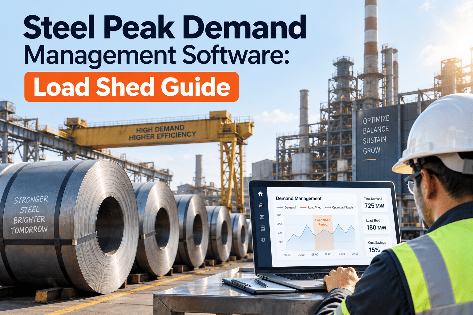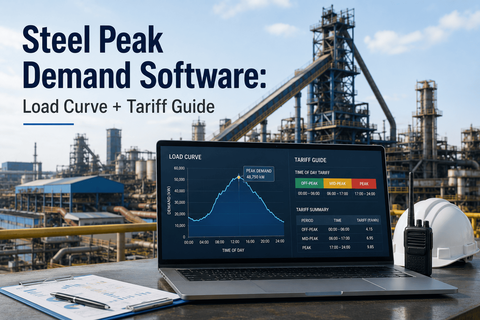
A single fifteen-minute window can set the electricity bill for an entire month, and most steel plants never see it happen — three large motors start within the same interval, a furnace and a compressor load together, and the coincident peak that results gets billed at a rate several times higher than normal consumption for every kilowatt in it. Demand charges routinely make up thirty to seventy percent of a large industrial user's electricity bill, and unlike the energy charge, the demand charge is set by the single worst quarter-hour of the month, not the average. Plants running melt shops, rolling mills, and compressor houses on independent schedules are the ones most exposed, because nobody is watching whether their peak loads happen to start together. Steel plants that actually control this cost are not the ones with lower average consumption — they are the ones tracking load curve shape, start sequencing, and tariff windows inside the same system that schedules maintenance and production, which is exactly what plants build with the OxMaint CMMS platform. From there, peak demand becomes a scheduling discipline instead of a monthly surprise on the utility invoice.
Peak Demand Software for Load Curve & Tariff-Aware Scheduling
Track coincident peak windows, load curve shape, and equipment start sequencing against your utility tariff — so the worst fifteen minutes of the month stop deciding the whole bill.
Anatomy of a Demand Charge — Why the Worst 15 Minutes Costs the Most
Industrial tariffs split into an energy charge, billed per kilowatt-hour consumed, and a demand charge, billed per kilowatt of peak power drawn in a single short interval. The demand charge is set by your maximum, not your average — one coincident spike from equipment starting together can cost the plant for the entire month, even though it lasted fifteen minutes on one morning. The four components below make up that exposure.
Non-Coincident Peak
The plant's own single highest demand interval in the billing period, regardless of what the wider grid is doing at that moment. Driven entirely by internal scheduling.
Coincident Peak
The plant's demand during the utility or grid operator's system-wide peak window, billed at a premium rate that can run several times the standard demand rate.
Load Factor
Average demand divided by peak demand. A low load factor means the plant pays for capacity it rarely actually uses — the clearest sign that scheduling, not consumption, is the real cost driver.
Ratchet Clause
Many tariffs carry forward a percentage of the peak demand from prior months as a minimum billing demand, meaning one bad peak can inflate bills for months afterward.
Flat Load Curve vs Spiked Load Curve — What Scheduling Actually Changes
Two plants can consume the exact same total energy in a month and pay very different demand charges, purely based on the shape of their load curve. The comparison below shows what changes when large loads are staggered instead of left to start on their own schedule.
Spiked Load Curve
Melt shop furnace, compressor bank, and rolling mill drives happen to start within the same quarter-hour on multiple mornings. Same total monthly energy, but the peak interval sets a demand charge far above what the plant's average operation actually requires.
Flattened Load Curve
Large motor and furnace start sequences staggered by a few minutes, and flexible loads shifted away from the utility's coincident peak window. Same production output, same total energy, materially lower peak demand charge.
Stop Paying a Month of Demand Charges for One Bad Quarter-Hour
OxMaint tracks load curve shape, equipment start sequencing, and tariff windows together, so scheduling decisions account for peak demand before the bill arrives.
Where Untracked Peak Demand Actually Costs a Steel Plant
Most plants track their total energy bill closely and their demand charge barely at all, even though the demand line item is often the larger and more controllable of the two. The breakdown below is where that cost typically concentrates once a plant starts separating the two charges.
Premium-rate charges from demand recorded during the utility's system-wide peak window, often unmanaged because it depends on grid timing, not just plant timing.
Large motors, furnaces, and compressors starting within the same interval by coincidence rather than design, setting an avoidable monthly peak.
Prior-month peak demand inflating current billing demand under ratchet clauses, extending the cost of a single bad interval across future months.
Paying for peak capacity that sits idle most of the month, the clearest sign that demand cost is a scheduling problem rather than a consumption problem.
Live Shift Demand Board — What Tracked Load Scheduling Looks Like
The board below shows a working day on a steel plant with a melt shop, rolling mill, and utility compressor house, tracked against the day's demand profile and tariff windows in real time.
Unmanaged Demand vs Tariff-Aware Scheduling
Nearly every plant already knows its production schedule. The gap is whether that schedule is checked against the utility tariff and coincident peak windows before it runs, or only reviewed after the bill arrives. The comparison below is what plants typically see in the first billing cycles after connecting scheduling to demand tracking.
| Program Element | Unmanaged (Bill Review Only) | Tracked (Schedule-Aware) | Typical Impact |
|---|---|---|---|
| Peak-Period Demand | Set by coincidental equipment starts | Actively staggered and scheduled | Up to 50% peak reduction |
| Load Factor | Typically 0.5–0.6 on batch-heavy plants | 0.7 and above with coordinated scheduling | Better capacity utilisation |
| Coincident Peak Exposure | Unknown until the utility statement arrives | Tracked and flagged before it happens | Avoided premium charges |
| Ratchet Clause Impact | Carries forward every bad peak | Minimised by preventing the peak itself | Lower baseline billing demand |
| Total Electricity Cost | Reviewed monthly after the fact | Actively managed against schedule | Documented cost reduction |
The Six Practices Behind Disciplined Peak Demand Management
Steel plants that consistently hold demand charges down are not running less equipment — they are running the same six practices inside their CMMS, treating peak demand as a scheduling constraint on par with production sequencing rather than a finance department afterthought.
Load Curve Monitoring
Plant-wide demand tracked in near real time against the billing threshold, so a developing peak is visible before the interval closes, not after.
Coincident Peak Window Mapping
Utility or grid-operator peak windows logged against the schedule, flagging any planned start that falls inside a premium-rate interval.
Staggered Equipment Starts
Large motors, furnaces, and compressors sequenced with a deliberate interval between starts, the single cheapest lever for cutting coincidental peaks.
Load Factor Trending
Average-to-peak ratio tracked over time, surfacing whether scheduling discipline is actually improving capacity utilisation or drifting back to old habits.
Ratchet Clause Review
Prior-period peaks checked against the current billing demand floor, quantifying exactly how long one bad interval will keep costing the plant.
Flexible Load Shifting
Non-time-critical maintenance runs and auxiliary loads moved outside peak windows wherever production sequencing allows.
What Tariff-Aware Scheduling Returns Across a Billing Year
The figures below reflect what steel plants typically document after connecting load scheduling to tariff and demand tracking, compounding across every billing cycle once the discipline is in place.
Peak-period demand reduced through optimal load scheduling and staggered equipment starts, documented across steel plant case studies.
Average-to-peak demand ratio improved as coincidental starts get deliberately staggered instead of left to chance.
Fewer bad peaks means fewer months where a ratchet clause carries forward an inflated billing demand floor.
Demand exposure flagged during scheduling instead of discovered a month later on the utility statement.
Frequently Asked Questions
Your Load Curve Shape Is a Scheduling Decision, Not a Utility Surprise
The steel plants keeping demand charges under control all track load curve, start sequencing, and tariff windows in one system — start managing your peak before it manages your bill.