Anomaly Detection: On-Prem AI for Real-Time Operations
By Riley Quinn on May 4, 2026
At 03:47 on a Tuesday, a 12,000-rpm centrifugal compressor at a chemical plant started vibrating 0.3 mm/s above its baseline. No threshold alarm tripped — it was inside the limit. Eleven days later, the bearing seized, taking the line down for 94 hours and costing $2.1M. A machine-learning anomaly model running on the same sensor stream flagged the drift at 03:51 — four minutes after it started — with 91% confidence of bearing degradation within 14 days. That four-minute gap is what real-time anomaly detection is actually selling. Static thresholds catch failures that have already started. Real-time AI catches the deviation that becomes the failure. Sign up free to see the anomaly detection pipeline running on your sensor data.
MAY 12, 2026 5:30 PM EST , Orlando
Upcoming OxMaint AI Live Webinar — Anomaly Detection On-Prem: From Sensor to Alert in Under 200 ms
Live session for reliability engineers, plant CIOs, control-systems leads, and AIOps teams. We'll architect a complete on-prem anomaly detection pipeline — sensor ingestion to streaming feature extraction, autoencoder scoring on GPU, traffic-light severity, automated work-order creation — at production-grade latency. Includes the false-positive reduction patterns that take rule-based alarms from "ignored" to "trusted."
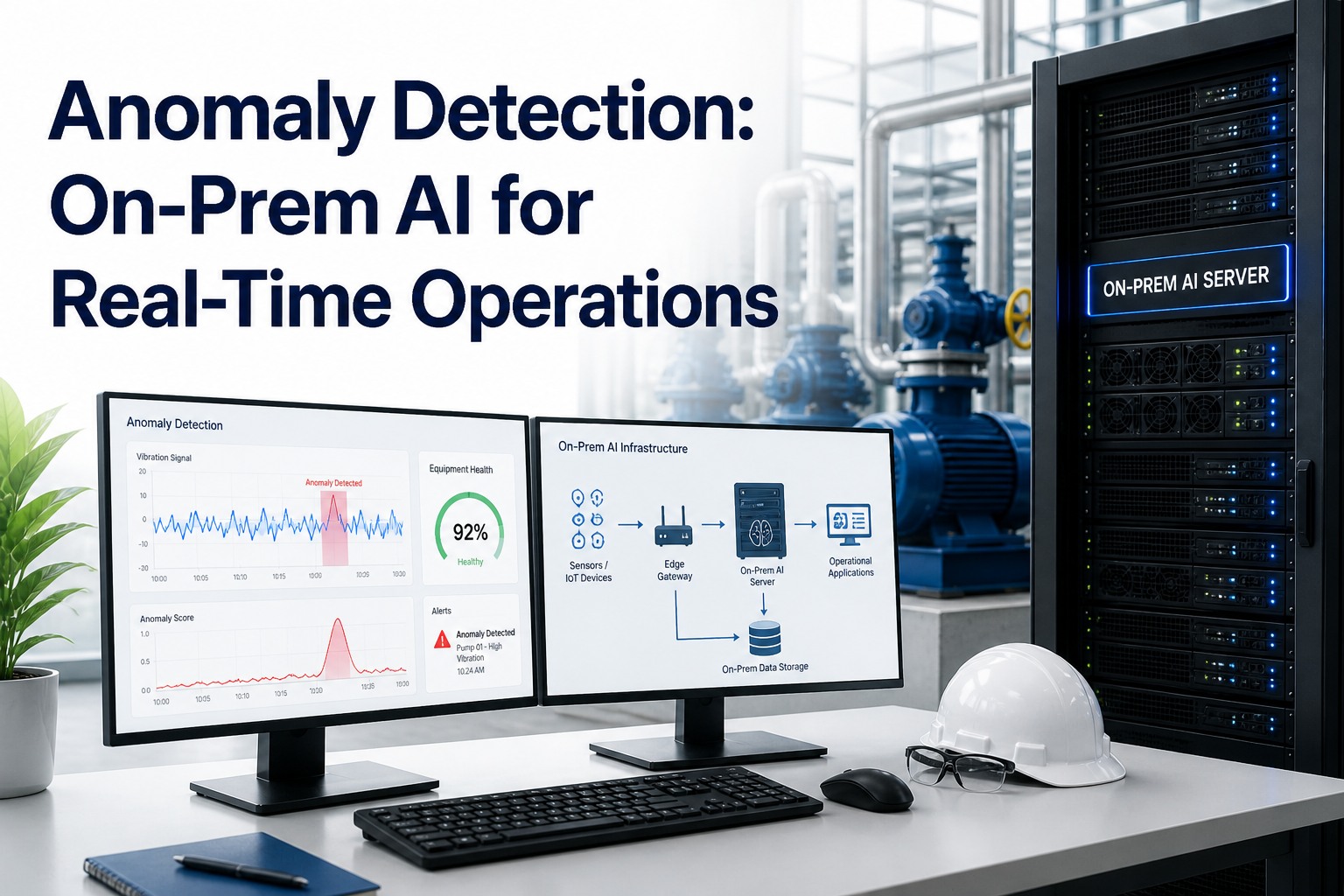
The Six-Stage Pipeline — Sensor to Alert in Under 200 ms
Real-time anomaly detection isn't one model — it's a pipeline. Every stage has a latency budget, a data-volume reality, and a place where it either runs on-prem or breaks. Here's the actual six-stage flow that production-grade industrial anomaly detection runs in 2026, with the numbers each stage handles.
01
Sensor Ingestion
Vibration, temperature, pressure, current, acoustic. Sample rates 1 Hz to 25 kHz. Modern plants generate 1–4 GB/asset/day. Edge agents compress and forward via MQTT or OPC-UA.
Latency budget5 msWhere it runsEdge / sensor side
02
Stream Buffer
Kafka or Redpanda buffers the firehose. Partitioned by asset. Out-of-order events handled. Decouples sensor side from model side — failures in one don't cascade.
Latency budget10 msWhere it runsOn-prem broker
03
Feature Extraction
FFT for frequency-domain features, wavelets for transient events, statistical aggregates per sliding window. Reduces 25,000 raw points to ~60 informative features the model can score against.
Latency budget40 msWhere it runsCPU on-prem
04
Model Inference (GPU)
Autoencoder reconstructs the feature vector. Reconstruction error becomes the anomaly score. Trained on 30–90 days of healthy operation per asset. Outputs probability + confidence interval.
Latency budget80 msWhere it runsGPU on-prem · <200 ms total
05
Traffic-Light Severity
Score classified into Green / Amber / Red. Green: normal. Amber: monitor. Red: action required. Adaptive thresholds adjust per asset based on operating context (load, ambient temp, duty cycle).
Latency budget5 msWhere it runsOn-prem rules engine
06
CMMS Action
Red anomaly auto-creates a work order with the spectral data attached, recommended action, and asset history. Routed to the right technician via mobile push. From sensor drift to work order in < 1 second.
Latency budget60 msWhere it runsCMMS · async push
Static Thresholds vs ML Anomaly Detection — Same Event, Two Outcomes
The defining distinction in 2026 industrial reliability is between static threshold alarms (legacy condition monitoring) and real-time ML anomaly detection (true predictive maintenance). Both watch the same sensor, both log the same data — and they produce radically different outcomes on the same physical event. Here's a real bearing-degradation timeline through both lenses.
T+0T+4 daysT+8 daysT+11 days
STATIC THRESHOLD
"Alert if vibration > 5 mm/s"
Drift unnoticed — still inside limit
ALARM
FAIL
94 hr line-down · $2.1M loss
ML ANOMALY DETECTION
Autoencoder, dynamic baseline per asset
OK
Amber — drift detected, schedule planned
Red — action ordered
DETECT
Scheduled service · 0 hr unplanned · $11K repair
67%fewer false positives vs rule-based alarms
94%detection accuracy on vibration data with deep learning
8–14 daystypical early-warning window before failure
The Three Algorithms That Actually Ship — And When to Use Each
"AI anomaly detection" covers a wide bench of algorithms. In production-grade industrial deployments, three patterns dominate — and the choice between them isn't preference, it's matched to the data shape. Book a demo to see all three running side-by-side on real plant data.
Isolation Forest
Batch
StrengthFast on tabular features, no labeled data required
Use whenMultivariate sensor features, periodic batch retraining acceptable
Trained on3–7 days minimum of healthy operation
Best forPumps, motors, fans — well-defined operating envelopes
Use whenMany correlated sensors, complex normal behavior, GPU available
Trained on30–90 days of healthy operation per asset
Best forCompressors, turbines, large rotating equipment with seasonal load
LSTM / Time-Series
Streaming
StrengthModels temporal dependencies, captures process drift
Use whenStrong time-of-day or shift seasonality, gradual drift detection
Trained on2–6 months of seasonal data preferred
Best forProcess equipment, HVAC, batch reactors, demand-driven assets
Why Anomaly Detection Goes On-Prem — Three Forces That Decide
The cloud-vs-on-prem question for anomaly detection has a clearer answer than most AI workloads. Three forces consistently push real-time anomaly detection on-prem regardless of vertical — and the engineering teams that recognize these early avoid the expensive rebuild after a cloud-only pilot fails to scale. Sign up free to see the on-prem anomaly stack designed for your sensor footprint.
Latency Reality
Sub-200 ms total pipeline budget. Cloud round-trip alone consumes 80–150 ms before the model runs. On a degraded WAN, latency variance is the killer — not the average. On-prem inference returns scores in < 80 ms with zero tail-latency surprise.
Data Volume Math
1–4 GB per asset per day. A 200-asset plant generates 200–800 GB/day of raw sensor data. Streaming all of that to the cloud is bandwidth cost that compounds linearly with sensor density. On-prem feature extraction collapses 25,000 raw points to 60 features before anything leaves the building.
Air-Gap & Sovereignty
Defense, energy, pharma, and critical-infrastructure sensors live on networks that don't reach the public internet by design. On-prem anomaly detection is the only architecture that meets the air-gap requirement — the sensor, the model, and the alert all stay on the same side of the firewall.
Pre-Configured · Pipeline-Ready · Ships in 6–12 Weeks
Order an Anomaly Detection Stack That's Trained Before It Arrives
OxMaint's anomaly detection AI server arrives pre-configured with the streaming buffer, feature extraction pipeline, autoencoder + Isolation Forest + LSTM model library, traffic-light severity engine, and CMMS work-order integration. Pre-configured, pre-tested, and ready to plug into your sensor network within days. Pre-trained on synthetic industrial data; production fine-tuning on 30–90 days of your healthy operation.
What an On-Prem Anomaly Detection Deployment Actually Costs
Most anomaly detection vendors charge per asset, per sensor channel, per stream — recurring, indefinitely, scaling linearly with your sensor density. The OxMaint anomaly detection stack is a one-time capital purchase: hardware, perpetual software license, AI models, streaming pipeline, and CMMS integration. No recurring license fees. Future costs are entirely optional and at your discretion. Sign up free to see anomaly detection pricing tailored to your asset count.
Swipe to see breakdown
Component
Unit Cost
Per Site (4 mo)
Notes
AI server (GPU + compute)
$19,000
$19,000
Autoencoder + LSTM inference, model retraining
Edge ingestion unit
$4,000
$4,000
Sensor protocol bridge — MQTT, OPC-UA, Modbus
Network + install
$10,500–$14,500
~$12,500
Plant VLAN, sensor cabling, electrical
OxMaint AI software + integration
$35,000–$55,000
$45,000 avg
Perpetual license, model library, CMMS integration, streaming pipeline
Per-Site Total
$72,500–$94,500
~$84,500 avg
4-month delivery — single plant or facility
4-Site Network Rollout
~$420,000–$520,000
Total programme
Parallel deployment across multiple plants
$84.5K
Avg per site
4 mo
Delivery
$0
Recurring fees
∞
Perpetual
The Numbers Industrial Reliability Teams Actually Care About
Marketing copy about anomaly detection talks about "AI-powered insights." Reliability engineers want hard numbers — what does the model catch, how often is it wrong, and how soon can the team trust the alerts. Here are the 2026 benchmarks from production deployments across manufacturing, energy, aviation, and process industries. Book a demo to see these benchmarks reproduced on your specific equipment.
94%
Detection accuracy on vibration data with deep learning anomaly models
67%
Reduction in false positives versus rule-based threshold alarms
8–14 days
Average early-warning window before catastrophic equipment failure
40%
Reduction in unscheduled equipment removals reported by GE Aviation on jet engines
30% / 50%
Maintenance cost reduction / downtime decrease reported by Siemens deployments
$98B
Predictive maintenance market size — anomaly detection is the technical backbone
Perpetual · Owned · Pre-Trained Pipeline · Ready to Run
Stop Waiting for Threshold Alarms to Catch Failures Already In Progress
A complete on-prem anomaly detection platform on enterprise-grade hardware in your plant. Streaming pipeline, feature extraction, autoencoder + Isolation Forest + LSTM model library, traffic-light severity, CMMS work-order integration — all pre-installed, all owned. No SaaS lock-in. No per-asset recurring fees. Source code and modification rights included.
How long does it take for the anomaly detection model to start producing reliable alerts?
It depends on the algorithm and the asset complexity. Isolation Forest models can produce useful alerts after 3–7 days of healthy-operation training data — these work well for pumps, motors, and fans with well-defined operating envelopes. Autoencoder models typically need 30–90 days of healthy operation data before they produce stable alerts at production-grade false-positive rates — these work best for compressors, turbines, and large rotating equipment with seasonal load. LSTM time-series models prefer 2–6 months of seasonal data to capture day-of-week, shift, and demand-cycle patterns. The OxMaint platform ships with synthetic-data pre-training that gives you a working model on day one, then progressively fine-tunes against your specific assets as healthy-operation data accumulates. Most plants see meaningful alerts in week 1, trustworthy alerts (low false-positive rate) by week 4–6, and full-confidence alerts by week 12.
Can the anomaly detection pipeline run with our existing PLC, SCADA, or historian data?
Yes — and this is the most common deployment pattern. The OxMaint anomaly detection stack connects to existing OT data sources via standard industrial protocols: OPC-UA for modern SCADA, Modbus TCP for legacy PLCs, MQTT for IIoT sensors, and direct historian integration for OSIsoft PI, GE Proficy, and AVEVA. You don't need to install new sensors — the model trains on whatever signal data you already collect. Common starting points are vibration, temperature, current draw, pressure, and flow rate. The data flows through the streaming buffer (Kafka or Redpanda), then through feature extraction, then into the model. The pre-configured connectors handle the common protocol translations; custom integrations to in-house OT systems typically take 1–2 weeks with the source-access pattern.
How does this avoid the false-positive problem that killed our previous anomaly detection pilot?
False positives are the most common reason anomaly detection pilots fail — alerts get ignored after the first week, and the system becomes shelfware. The OxMaint pipeline addresses false positives at three layers. First, multivariate detection means the model needs multiple correlated signals to deviate before flagging — single-channel transients (cable movement, sensor noise, external vibration) get filtered. Second, adaptive thresholds adjust per asset based on operating context (load, ambient temp, duty cycle) — so a vibration spike during high load doesn't trigger if it's normal for that load level. Third, the traffic-light severity (Green / Amber / Red) gives operators graduated alerts — Amber is "monitor, no action required," which keeps the alert volume realistic. Production deployments typically see 67% fewer false positives versus rule-based threshold alarms within the first 4–6 weeks of model maturation. Each closed work order also feeds back into the model, so false positives decline over time as the system learns which alerts produce real findings.
What's the difference between OxMaint anomaly detection and the AIOps tools we already use?
AIOps platforms (Datadog, New Relic, Dynatrace, Splunk Observability) are designed for IT infrastructure anomaly detection — server metrics, application latency, log patterns, distributed traces. They're excellent at what they do, and many also offer rule-based and ML-based alerting. The OxMaint platform is designed for operational technology (OT) anomaly detection — physical equipment, vibration spectra, process variables, sensor fusion. The data shapes are different (high-frequency time-series sensor signals vs structured logs and metrics), the models are different (autoencoders on FFT features vs Isolation Forest on log frequency), and the actions are different (CMMS work orders + technician dispatch vs Slack alerts + ticket creation). Most plants run both: AIOps for the IT side, OxMaint for the OT side. The OxMaint platform integrates with AIOps tools via webhooks for cross-domain incident correlation when the same root cause spans both sides — for example, a SCADA gateway failure showing up as both an IT metric anomaly and an OT data-loss anomaly.
How long from purchase to live anomaly detection on our equipment?
Six to twelve weeks from sign-up to live operation is typical. The compressed timeline works because the server is configured, integrated, and pre-tested in the OxMaint factory before shipping — GPU, AI software, model library (autoencoder, Isolation Forest, LSTM), streaming pipeline (Kafka), feature extraction, and CMMS connectors are all installed and validated against synthetic industrial data before the unit ships. On-site work then collapses to: rack the server in your data center or plant control room (1 day), connect to your SCADA/PLC/historian (2–3 days), configure asset list and sensor mapping (1 week), pre-train models on existing healthy-operation data (1–2 weeks, runs in parallel), validate alerts in shadow mode against current operations (2–4 weeks), then production cutover. Most plants run the system in shadow mode (alerts logged but not auto-creating work orders) for the first month to build operator confidence before enabling automatic CMMS integration.