Vibration Analysis 101: Diagnosing Bearing Failures Before They Stop Production
By Riley Quinn on May 6, 2026
Every rolling-element bearing fails the same way: it tells you it's dying for nine months before it actually stops the line. The only question is whether anyone is listening. Around month nine, ultrasound starts hearing micro-cracks no one notices. Around month six, vibration analysis spots subtle peaks at frequencies the bearing literally calculates from its own geometry. Around month three, the noise becomes audible to a trained ear. Around month one, the bearing housing gets warm enough to feel. Around hour zero, it seizes mid-shift and takes the line down. The window between the first detectable signal and functional failure is called the P-F interval, and modern AI-driven vibration analysis stretches that window from "weeks of warning" to "months of warning" — long enough to schedule the repair instead of scrambling for it. Sign up free to run the bearing fault decoder on your equipment data.
MAY 12, 2026 5:30 PM EST , Orlando
Upcoming OxMaint AI Live Webinar — Vibration Analysis 101: Diagnosing Bearing Failures Before They Stop Production
Live session for reliability engineers, maintenance managers, vibration analysts, and operations teams building modern condition-monitoring programs. We'll walk through the P-F curve in detail, decode the four bearing fault frequencies (BPFO, BPFI, BSF, FTF) with worked examples, demonstrate how AI-powered envelope analysis catches Stage 1 bearing defects six to nine months before failure, and show the OxMaint AI Vision Camera deployment that ships pre-trained and ready to run in 6–12 weeks.
The P-F Curve — The Reliability Engineer's Universal Map
The P-F curve is the diagram every reliability engineer learns in week one of training, and it's the single most useful framework for understanding why some maintenance programs catch failures and others don't. The horizontal axis is time. The vertical axis is asset condition. The curve starts flat (healthy operation), tilts down at point P when the failure begins to develop, and crashes down to point F when the asset stops doing its job. Every detection technology has a position on this curve — the further left it can detect, the more time you have to plan a repair. For bearings, the order is the same in every plant.
9 mo
Vibration analysis catches the earliest defect signal — bearing micro-spalls excite resonance frequencies that show up in envelope-demodulated FFT spectra.
3 mo
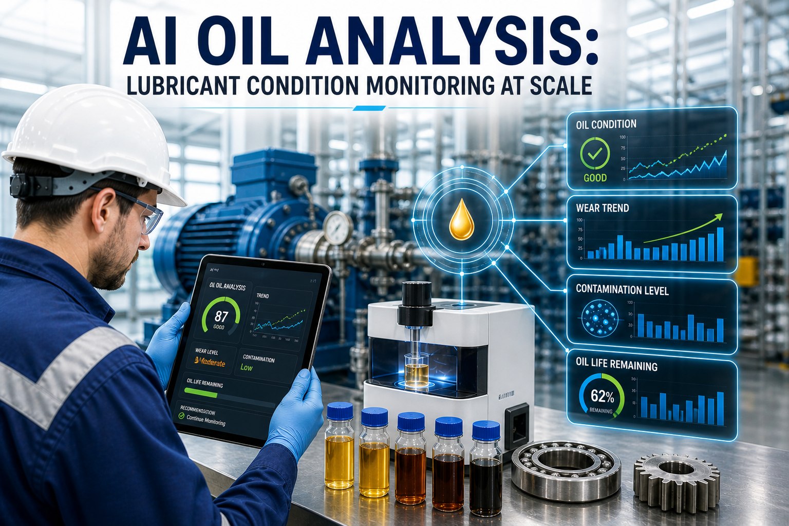
Oil analysis detects metallic wear particles in the lubricant. Late-stage indicator — by the time particles are circulating, mechanical damage is well underway.
1 mo
Audible noise — the bearing now whines or rumbles loud enough for a trained ear. Repair window has shrunk from months to weeks.
1 wk
Heat & smell — touch-temperature, lubricant burn smell. Final warning. Fix it now or it stops production within days.
The Four Bearing Fault Frequencies — Read the Bearing's Geometry
Here's the magic that makes bearing diagnostics possible: every defect generates a vibration at a frequency you can calculate from the bearing's geometry alone. A spall on the outer race produces a peak at exactly BPFO. A crack on the inner race produces a peak at exactly BPFI. The geometry doesn't lie — if your spectrum has a sharp peak at the calculated BPFO frequency, you have outer-race damage. Period. The four formulas below are the toolkit every certified Category I vibration analyst memorizes; modern AI analyzers compute them automatically and watch for amplitude growth at each frequency over time. Book a demo to walk through bearing fault frequency decoding running on your equipment.
BPFO
Ball Pass Frequency · Outer Race
≈ 0.4 × Nb × RPM ⁄ 60
Most common bearing failure mode
Outer race is stationary, so the defect sits in a fixed load-zone position. Each rolling element passing over the spall produces an impact at exactly this frequency. Easiest of the four to detect.
SKF 6205 @ 1,800 RPM (9 balls)
≈ 108 Hz
BPFI
Ball Pass Frequency · Inner Race
≈ 0.6 × Nb × RPM ⁄ 60
Always higher than BPFO
Inner race rotates with the shaft, so the defect moves through the load zone, modulating amplitude at 1× RPM. Produces 1× sidebands around BPFI — the unmistakable inner-race signature.
SKF 6205 @ 1,800 RPM (9 balls)
≈ 162 Hz
BSF
Ball Spin Frequency · Rolling Element
≈ 0.23 × Nb × RPM ⁄ 60
Hardest of the four to detect
Rolling element rotates on its own axis. A defect strikes both races each revolution, producing a peak at 2× BSF. Slip between elements and races smears the signal — envelope analysis essential.
SKF 6205 @ 1,800 RPM (9 balls)
≈ 62 Hz
FTF
Fundamental Train Frequency · Cage
≈ 0.4 × RPM ⁄ 60
Sub-synchronous (below 1× RPM)
The cage rotates at 0.4× shaft speed. Cage damage, retainer wear, or bearing-induced rotor instability produces a peak below 1× RPM. The only sub-synchronous bearing fault — a distinctive signature.
SKF 6205 @ 1,800 RPM
≈ 12 Hz
The Four Stages of Bearing Failure — Watch the Spectrum Change
Bearings don't fail all at once. They progress through four well-documented stages, and each stage produces a distinct vibration spectrum that's recognizable to a trained analyst (or a properly trained AI model). The horizontal timeline below shows what an FFT spectrum actually looks like at each stage, when each stage typically occurs relative to functional failure, and what action a reliability program should take. Sign up free to load your bearing data into the four-stage classifier.
STAGE 1
6–9 months from failure
Sub-Surface Initiation
Micro-cracks below the race surface. Standard FFT shows nothing. Only ultrasonic / high-frequency envelope detection methods (PeakVue, Spike Energy, SEE) catch it.
Action: trend only · no immediate response needed
STAGE 2
1–6 months from failure
Resonance Excitation
Defects begin exciting bearing component natural frequencies (typically 500 Hz – 2 kHz). Distinct hump appears in mid-frequency range. Defect frequencies still buried.
Action: plan repair · monitor monthly
STAGE 3
2–8 weeks from failure
Defect Frequencies Visible
Defect frequencies (BPFO/BPFI/BSF/FTF) and harmonics now dominate the spectrum. Sidebands at 1× RPM appear. The textbook diagnostic stage — clean, unambiguous, actionable.
Action: replace at next scheduled outage
STAGE 4
Days to weeks from failure
Random High-Frequency Noise
Defects round off, clearances grow, looseness dominates. Discrete peaks fade as broadband noise rises across the spectrum. 1× RPM amplitude climbs sharply.
Action: emergency shutdown, replace immediately
How AI Adds 6 Months to the Detection Window
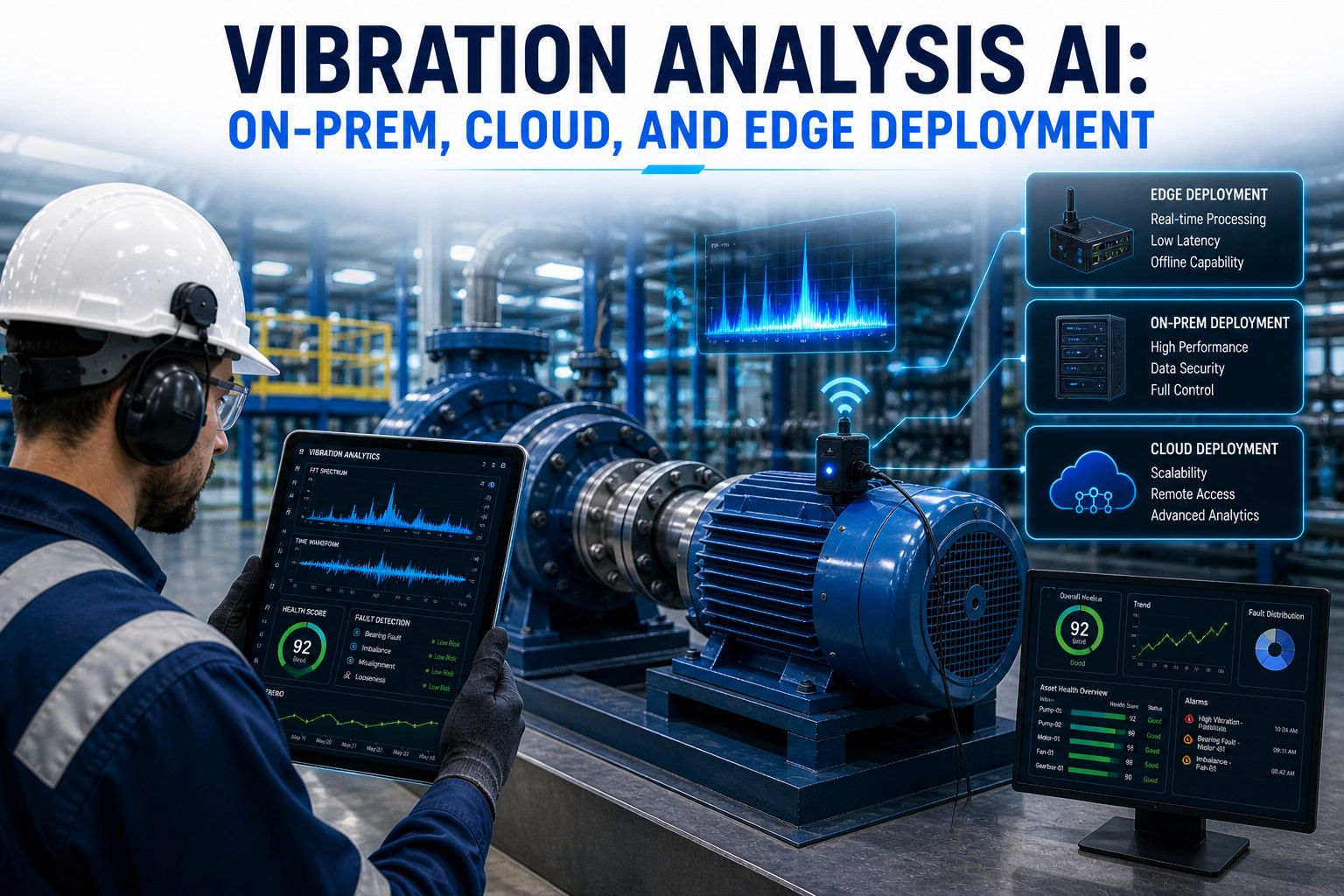
Traditional vibration programs use route-based monitoring — a technician walks a fixed list of bearings monthly with a handheld analyzer, manually interprets the spectrum, makes a judgment call. The system works, but it has three structural limits: humans get tired, monthly intervals miss faults with shorter P-F windows, and judgment quality varies by analyst experience. AI vibration analysis solves all three. Continuous wireless sensors capture data 24/7. AI models trained on millions of fault spectra match patterns instantly. Trend detection catches subtle envelope-spectrum changes that point to Stage 1 defects months before a human would spot them.
Traditional · Monthly Route
2-3 months avg detection lead time
~3 mo
Continuous Wireless · Manual Review
5-6 months avg detection lead time
~6 mo
AI-Powered · Continuous + Envelope
9 months avg detection lead time · Stage 1 sensitivity
~9 mo
The 6-month gap matters: at 3 months you scramble for parts and overtime. At 9 months you order the bearing on standard lead time, schedule the work into a planned outage, and the line never stops.
Owned, Not Rented — The OxMaint AI Vibration Stack
The OxMaint AI Vibration deployment isn't a SaaS subscription you pay every month forever. It's a pre-configured AI server bundled with wireless triaxial accelerometers, AGX Orin edge appliances for envelope analysis at the sensor edge, and an RTX PRO 6000 Blackwell server running the FFT analyzer, fault classifier, and CMMS connector. Pre-trained on the four-stage bearing failure library. Get a quote and order it like the hardware it is — pre-configured, pre-tested, ready to run within days of installation, and owned outright the day delivery completes.
Perpetual License
No monthly fees, no per-sensor metering, no per-asset billing. Future costs are entirely optional and at your discretion.
Data Sovereignty
Vibration spectra, FFT data, bearing fault classifications all live on your server, behind your firewall. Never uploaded.
Source Access
Source code and modification rights included. Add custom bearing geometries, retrain fault classifiers, integrate freely.
AI-Native Core
FFT analysis, envelope demodulation, four-stage fault classification, NLP work orders — built in, not bolted on.
Pre-Configured · FFT-Ready · Ships in 6–12 Weeks
Order an OxMaint Vibration Analysis Stack — Pre-Loaded
A complete on-prem AI vibration deployment for bearing fault detection. Wireless triaxial accelerometers, AGX Orin edge appliances running envelope analysis, RTX PRO 6000 Blackwell central server running FFT spectrum analyzer plus four-stage bearing fault classifier, automatic CMMS work-order generation when defect frequencies cross threshold. Pre-trained on industrial bearing fault datasets, ready to fine-tune on your specific equipment within days.
From Spectrum to Work Order — The Closed-Loop Pipeline
Catching a Stage 2 bearing fault isn't the deliverable. The deliverable is a scheduled bearing replacement during planned downtime, with the right bearing on the shelf, the right technician assigned, and the right CMMS history attached. The OxMaint AI Vibration Stack connects every detection directly to the CMMS work-order engine, with rule logic that maps each fault stage to its standard corrective procedure. Book a demo to walk through the spectrum-to-work-order pipeline on your assets.
01
Sense
Wireless triaxial accelerometers stream 25.6 kHz vibration data continuously. Battery life 5+ years on standard mounting.
The OxMaint AI Vibration Stack uses the standard per-plant architecture: central RTX PRO 6000 Blackwell server plus two AGX Orin edge appliances, with wireless triaxial accelerometers added per critical asset. FFT analysis, envelope demodulation, four-stage bearing fault classification, and CMMS connectors all included in the OxMaint AI Software + Integration line. Sign up free to walk through per-plant pricing for your bearing footprint.
Swipe to see breakdown
Component
Unit Cost
Per Plant
Notes
RTX PRO 6000 Blackwell 96GB Server
$19,000
$19,000
FFT analyzer + Synapse AI fault classifier
NVIDIA AGX Orin #1 (Sensor Edge)
$4,000
$4,000
Envelope demodulation + sensor aggregation
NVIDIA AGX Orin #2 (PLC + CCTV Edge)
$4,000
$4,000
PLC tag sync + CCTV inference
Industrial Ethernet Switch + Cabling
~$2,500
~$2,500
Plant-floor switch, Cat6A, SFP modules
Local Electrical / Instrumentation
$8,000–$12,000
~$10,000 est
Sensor mounting, wireless gateway, conduit
OxMaint AI Software + Integration
$35,000–$55,000
$45,000 avg
Bearing models, CMMS connectors, training
Per-Plant Total
$72,500–$94,500
~$84,500 avg
4-month delivery per plant
4-Plant Full Rollout (with Enterprise AI)
~$420,000–$520,000
Total programme
Parallel delivery + DGX Station GB300 Ultra
$84.5K
Avg per plant
4 mo
Delivery
$0
Recurring fees
∞
Perpetual
Perpetual · Owned · Source Access · Data Sovereignty
Stop Catching Bearings at Stage 4 — Detect at Stage 1, Owned
FFT spectrum analysis, envelope demodulation, four-stage bearing fault classification, automatic CMMS work-order generation, and the full OxMaint software stack. Your team owns the platform, the AI models, and the source code outright. The architecture every modern reliability program is converging on as bearings move from reactive to truly predictive.
What's the difference between vibration analysis and envelope analysis?
Vibration analysis is the broad discipline of measuring and interpreting machine vibration. The standard tool is the FFT (Fast Fourier Transform), which converts a time-domain vibration signal into a frequency-domain spectrum showing peaks at characteristic frequencies. Envelope analysis is a specialized technique within vibration analysis specifically designed to extract bearing defect signatures. The problem with raw FFT for bearings is that defect impulses are short, sharp, and high-frequency — they get buried under low-frequency dominant peaks (1× RPM unbalance, 2× misalignment, gear mesh frequencies). Envelope analysis applies a high-pass filter to isolate the high-frequency band where bearing defects live (typically 1-20 kHz), demodulates the amplitude envelope to extract the impact rate, then runs FFT on that envelope. The result: a clean spectrum showing exactly the bearing defect frequencies (BPFO/BPFI/BSF/FTF) without contamination from rotor faults. Modern AI vibration systems run both in parallel — raw FFT for general fault diagnosis, envelope analysis for early-stage bearing detection.
How accurate are the simplified BPFO/BPFI formulas?
The simplified approximations (BPFO ≈ 0.4 × Nb × RPM/60, BPFI ≈ 0.6 × Nb × RPM/60) are typically accurate to within ±5% for most common rolling-element bearings — good enough for field diagnostics when the bearing manufacturer's geometric data isn't available. The exact formulas use the bearing's pitch diameter (Pd), ball diameter (Bd), contact angle (α), and number of rolling elements (Nb): BPFO = (Nb/2) × (RPM/60) × [1 - (Bd/Pd) × cos α] and BPFI = (Nb/2) × (RPM/60) × [1 + (Bd/Pd) × cos α]. The sign difference between the two formulas is what creates the BPFI > BPFO relationship. For formal analysis reports and trending programs, always use the exact formulas with manufacturer-supplied geometry. The OxMaint AI Vibration Stack ships with a database of 2,700+ bearing geometries pre-loaded (SKF, NTN, Cooper, Dodge, FAG, NSK, Timken, and others) so the exact frequencies are calculated automatically once a bearing part number is entered.
Why does bearing damage often appear at harmonics, not just the fundamental?
A spall or crack on a bearing race produces a sharp impact every time a rolling element rolls over it. That impact is broadband — it contains energy at the fundamental defect frequency plus integer multiples (2×, 3×, 4×, ...). In Stage 2 of bearing failure, you typically see the fundamental peak alone. In Stage 3, you see the fundamental plus 2× and 3× harmonics with progressively decreasing amplitude. By late Stage 3, you may see 4-6 harmonics, and the relative amplitudes of the harmonics tell you about the defect geometry. Sharp narrow defects produce many strong harmonics. Wide rounded defects produce fewer harmonics. Additionally, inner-race defects produce sidebands at 1× RPM around BPFI and its harmonics — that sideband pattern is the textbook BPFI signature. AI fault classifiers don't just look for the fundamental peak; they look at the full harmonic and sideband pattern to determine fault stage and projected remaining useful life.
Should I use ISO 10816 vibration severity charts?
ISO 10816 (now updated as ISO 20816) gives you broadband vibration severity zones that are useful as a starting point — Zone A (good), Zone B (acceptable for unrestricted long-term operation), Zone C (unsatisfactory for long-term operation), Zone D (severe enough to cause damage). The standard breaks machines into classes based on power and rigidity, and the threshold values (in mm/s RMS) are different per class. The honest framing is that ISO severity charts catch overall vibration trends but miss the specific bearing fault frequencies — a bearing in early Stage 2 with developing BPFO might still pass ISO Zone A because the broadband RMS is low. Modern reliability programs use ISO charts as the alarm-level overview plus FFT spectrum analysis with envelope demodulation as the diagnostic depth. The OxMaint AI dashboard shows both: ISO severity zones for instant fleet-wide health overview, plus drill-down spectrum analysis when something crosses threshold.
How long until our reliability team is productive with AI vibration analysis?
Most reliability teams reach basic productivity within 2-3 weeks of deployment and full diagnostic fluency within 2-3 months. The OxMaint AI Vibration Stack includes structured training: weeks 1-2 cover sensor mounting, FFT basics, and the four bearing fault frequencies; weeks 3-4 cover envelope analysis interpretation and the four-stage failure model; weeks 5-8 cover advanced diagnostics including combined-fault separation, sideband analysis, and integration with existing Category I/II vibration analyst workflows. Teams already running Category I/II vibration programs typically ramp faster — they recognize the spectrum patterns immediately and just need to learn the OxMaint interface. Teams new to vibration analysis benefit from the AI pre-classification which reduces the cognitive load of spectrum interpretation. By month 4, the plant team is independently operating the AI Vibration Stack with thresholds tuned to plant conditions, custom bearing geometries added for legacy equipment, and CMMS work orders auto-generating from every above-threshold detection.