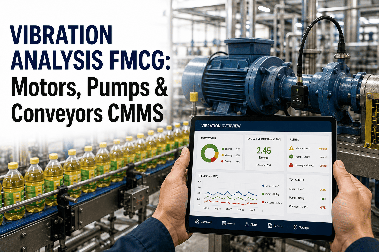
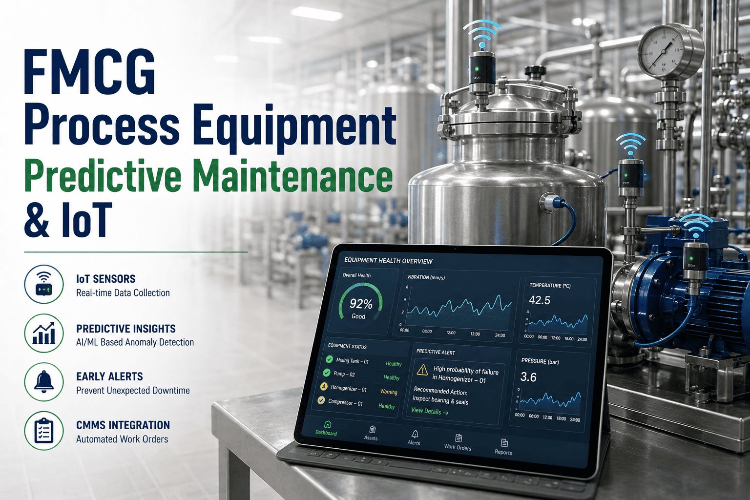
A snack food plant in Gujarat installed vibration sensors on 14 high-speed packaging lines in 2023. For the first three months the alerts were nearly useless — thresholds set from generic benchmarks bore no relationship to how those machines ran at 620 packs per minute in 38°C heat. Technicians learned to ignore them. Then the ML models had enough run-time data to learn what normal actually looked like for each machine, each shift, each season. By month six, the same sensor network was catching bearing degradation 19 days before failure — not because the sensors changed, but because the intelligence interpreting them had learned the difference. This is the core principle of ML for FMCG equipment: models learn the specific behavioral fingerprint of your assets and detect deviation from it. Oxmaint's ML platform connects to your existing IoT sensors and CMMS history and starts generating failure predictions within 2–4 weeks. Book a demo to see it applied to your equipment.
19
Days Average Bearing Degradation Lead Time — Gujarat Snack Plant After 6 Months of ML Model Maturity
75%
Reduction in False Positive Rate — Rule-Based Alerts vs. Mature ML Models on Same Sensor Network
14–28
Days Failure Prediction Lead Time at Model Maturity — Cross-Asset Average in FMCG Plants
5–12×
Return on ML Predictive Maintenance Investment — Combined Repair, Downtime, and Inventory Value
ML-Powered Predictive Maintenance — Live on Your Equipment
Your Equipment Already Has the Data. Oxmaint Has the Models.
Oxmaint's ML platform connects to your existing IoT sensors, BAS feeds, and CMMS history to learn your asset behavior — and starts generating failure predictions within 2–4 weeks of initial data ingestion. No data science team required.
RULE-BASED VS. ML
Rule-Based Alerts vs. Machine Learning — What Changes When AI Learns Your Assets
Why generic thresholds fail and how ML models trained on your specific equipment transform detection accuracy
Rule-Based / Fixed Threshold Alerts
Vibration Threshold
Fixed value from OEM manual — ignores product, speed, ambient conditions
Temperature Alert
Generic limit — fires on every summer startup, ignored by operators
False Positive Rate
35–60% — teams learn to ignore alerts, missing real failures
Failure Lead Time
0–3 days — alert fires when degradation is already severe
Seasonal Adaptation
None — same threshold year-round regardless of conditions
ML Models — Asset-Specific Learned Behavior
Vibration Baseline
Learned per machine, per speed setting, per product type — deviation flagged
Temperature Baseline
Normal range learned including startup curves, load cycles, seasonal variation
False Positive Rate
8–15% by month 6 — alerts carry credibility, teams respond
Failure Lead Time
7–28 days — degradation caught while repair is still planned and cheap
Seasonal Adaptation
Continuous — model relearns baselines as conditions change
Accuracy Improvement: Rule-Based → ML False Positives Drop 75% — Detection Lead Time Extends 6–9×
LEARNING CYCLE
Four-Stage ML Model Learning Cycle for FMCG Equipment
Stage 1
Data IngestionWeeks 1–2
Vibration, temperature, current draw, pressure, and speed data ingested from IoT sensors at configurable intervals
CMMS work order history imported — failure codes, repair dates, parts replaced — to anchor learning to known fault events
Operating context tagged: production run vs. idle, product type, line speed, ambient temperature
Data quality audit: sensor drift detection, gap filling, outlier identification before training begins
Output: Clean, context-tagged dataset ready for baseline learning
Stage 2
Baseline ConstructionWeeks 2–6
Normal operating envelopes built per asset, per operating mode — what does healthy vibration look like at 400 rpm vs. 620 rpm for this specific motor?
Temporal patterns learned: startup transients, warm-up curves, steady-state windows, shutdown signatures
Cross-parameter correlations established: temperature and current draw relationship under load
Seasonal baseline layers built as weeks accumulate — summer vs. winter operating norms captured
Output: Asset-specific normal behavior model — deviation now detectable
Stage 3
Anomaly DetectionMonth 2 onward
Real-time deviation scoring: every incoming sensor reading compared against learned baseline — deviation magnitude scored continuously
Multi-parameter anomaly fusion: correlated deviations across 3+ sensors trigger detection even below individual alert thresholds
Fault signature library matching: detected patterns compared against known failure precursors from CMMS history
Remaining useful life estimation: degradation trajectory projected forward to estimate time-to-failure window
Output: Prioritised alerts with failure timeline and confidence score
Stage 4
Continuous ImprovementOngoing
Every confirmed failure and near-miss updates the model — correct predictions reinforce the signature, false positives trigger recalibration
Maintenance action outcomes fed back: model learns optimal intervention timing from real repair results
Equipment modifications tracked: after rebuild, model resets baseline and learns the new post-repair norm
Cross-fleet transfer learning: failure patterns from one line inform detection on identical equipment elsewhere
Output: Accuracy compounds — prediction improves every month
SIGNAL CATEGORIES
Six Key ML Signal Categories in FMCG Equipment
Different failure modes produce different physical signatures — these six categories cover the dominant failure modes in FMCG production
Vibration Signatures
Bearing & Gear Faults
Frequency-domain analysis detects bearing spall, gear mesh degradation, imbalance, and misalignment. Each fault type produces a characteristic frequency signature — ML learns to distinguish these from normal vibration at each operating speed.
Thermal Patterns
Motor & Drive Health
Temperature rise curves, steady-state operating temperatures, and thermal gradients across motor frames reveal winding insulation degradation, cooling blockages, and overload conditions with 3–8 week lead time.
Current Draw Profiles
Load & Efficiency Drift
Motor current signatures encode mechanical load, rotor condition, and drive efficiency in real time. ML detects the gradual current increase that precedes bearing seizure and asymmetry patterns indicating stator winding faults.
Pressure & Flow Dynamics
Pump & Valve Condition
Pressure differential trends across filters and valves, pump discharge curves, and flow rate consistency expose seal degradation, impeller wear, and valve seat erosion weeks before product quality is affected.
Acoustic Emission
Lubrication & Crack Detection
Ultrasonic and acoustic sensors capture lubrication film breakdown at bearing surfaces, partial discharge in electrical systems, and micro-crack propagation — detecting failure precursors invisible to vibration analysis alone.
Cycle Time & Throughput
Mechanical Wear & Drag
Packaging line cycle times, servo positioning accuracy, reject rates, and throughput per hour encode mechanical wear and servo drive drift. ML detects the gradual performance decline operators normalise long before it becomes a measurable OEE loss.
ROBOTIC SELF-DIAGNOSTICS
What ML Monitors in FMCG Cobots and AMRs
Integrated sensor data that ML models analyse for health scoring and failure prediction
Joint Torque Signatures
Each cobot joint has a learned torque profile for every programmed motion path. Deviation indicates gearbox wear, lubrication loss, or path obstruction before joint failure.
4–10 Week Lead
Motor Encoder Drift
Position accuracy across thousands of repeat cycles — ML detects micro-drift in repeatability that indicates encoder degradation or mechanical backlash developing in the drive train.
6–12 Week Lead
AMR Wheel & Drive Health
Drive motor current, wheel encoder slip, and IMU-detected vibration reveal wheel wear and motor brush wear — AMR self-reports reduced traction before it affects navigation accuracy.
3–8 Week Lead
Payload & Path Anomalies
Unexpected torque loads detect tooling wear and gripper pressure decay. Unplanned path deviations on AMR routes indicate navigation sensor drift or obstacle detection calibration drift.
Real-Time Detection
Thermal & Power Monitoring
Controller temperature, battery state-of-health trending, and power supply voltage stability — ML detects degradation in power systems that precede unexpected shutdowns during production.
2–6 Week Lead
Vision System Calibration Drift
Camera-based inspection and navigation systems develop calibration drift over time. ML detects confidence score degradation before mis-detections affect quality outcomes.
Continuous Scoring
Cobots and AMRs with ML self-diagnostics reduce unplanned downtime by 71% compared to reactive repair — and because the equipment generates its own work orders, there is zero monitoring labour overhead.
AI/ML Analytics — Production-Ready for FMCG Assets
From Sensor Data to Failure Prediction in 4 Weeks
Oxmaint's ML models connect to your existing vibration, thermal, and current sensors — learn your equipment's behavioral fingerprint — and begin generating prioritised failure predictions with remaining useful life estimates within the first production month.
ACCURACY TRAJECTORY
ML Model Accuracy by Deployment Stage
Days 1–30: Fault Detection Mode
70–80% Fault Detection
Models operate in fault detection mode — identifying current operational problems like stuck valves and sensor drift rather than predicting future failures. Value is immediate but not yet predictive. False positive rate is typically 25–40% as baselines are still being established.
Days 30–90: Pattern Learning Phase
80–88% Prediction Accuracy
With 4–12 weeks of operational data, models have learned startup curves, shift-change patterns, and day/night thermal cycles. Predictive alerts now extend 7–14 days ahead. False positive rate drops to 15–25% as baselines solidify.
Day 90+: Full Predictive Operation
88–95% Prediction Accuracy
After 3+ months, models deliver production-grade prediction accuracy with 14–28 day lead times on critical assets. False positive rate stabilises at 8–15%. At 12 months, models typically achieve 90–95% accuracy on their primary monitored failure modes.
ASSET-BY-ASSET
ML Monitoring Matrix — FMCG Equipment Asset by Asset
What ML models learn, what failure signatures they detect, and the prediction lead time at model maturity
High-Speed Packaging Lines
Servo motor current signatures, cam follower vibration, jaw seal temperature, film tension variance, cycle time drift. Detects mechanical wear, seal degradation, and drive issues before speed loss or mispack incidents.
10–21 Days
Mixing & Blending Equipment
Agitator motor current under load, gearbox vibration spectrum, seal face temperature, torque fluctuation. Catches impeller imbalance, gearbox wear, and shaft seal degradation before product contamination risk.
14–28 Days
Filling & Dosing Systems
Fill head pressure consistency, valve cycle time accuracy, pump discharge flow curves, piston position encoder drift. Detects valve wear and pump degradation before fill weight drift fails quality checks.
7–18 Days
Conveyor & Transfer Systems
Drive motor current at load, belt tension via drive torque, idler bearing vibration signatures. Identifies belt stretch, bearing degradation, and drive chain wear before stoppage events.
14–35 Days
CIP & Cleaning Systems
Pump discharge pressure during CIP cycles, flow rate consistency at each spray head zone, chemical dosing pump stroke accuracy. Detects fouling, nozzle blockage, and pump degradation before hygiene compliance risk.
7–14 Days
Refrigeration & Cooling
Compressor suction/discharge pressure ratio, condenser approach temperature, refrigerant charge via superheat/subcool, compressor current draw efficiency index. Catches refrigerant loss and compressor valve wear before temperature excursions.
21–42 Days
Lead times above assume 90+ days of model maturity with sensor data quality above 85%. Assets with richer CMMS failure history achieve upper-range lead times faster — existing work order data accelerates baseline calibration by 3–6 weeks.
DATA REQUIREMENTS
ML Data Requirements — Minimum Viable vs. Optimal
END-TO-END WORKFLOW
ML Alert to Planned Repair — The Oxmaint Workflow
Step 1
Anomaly DetectedML Model
Deviation score crosses confidence threshold — multi-parameter anomaly confirmed across 2+ sensors on the same asset
Failure mode classified against known signature library — bearing spall vs. imbalance vs. misalignment each triggers different recommended action
Remaining useful life estimated — probability distribution of time-to-failure generated with high/medium/low urgency bands
Output: Structured alert with failure type, confidence, and urgency band
Step 2
Work Order CreatedCMMS Auto-Generation
Work order auto-generated in Oxmaint CMMS with asset ID, failure mode, urgency priority, and ML confidence score pre-populated
Recommended parts list pulled from CMMS parts master based on failure mode — parts availability checked against current inventory
Optimal intervention window suggested based on RUL estimate and production schedule
Output: Ready-to-action work order in maintenance queue
Step 3
Technician DispatchMobile Workflow
Technician receives work order on Oxmaint mobile app with asset location, failure context, recommended procedure, and parts list
AI copilot available for fault diagnosis support — query the anomaly data, compare to historical similar failures, get ranked diagnosis recommendations
Work completed with photo documentation, parts consumed recorded, and condition-at-inspection captured for model feedback loop
Output: Intervention completed with full documentation
Step 4
Model FeedbackContinuous Learning
Work order outcome — confirmed failure mode, component condition, repair action — fed back to ML model as a training label
Prediction accuracy scored: was the failure mode correct? Was the urgency band accurate? Each outcome calibrates the model
Cross-asset learning triggered: validated failure signatures shared across identical equipment models across sites
Output: Model improves — next prediction more accurate
ROI FRAMEWORK
ML Predictive Maintenance ROI — FMCG Plant Benchmarks
Value delivered per category — mid-size FMCG plant, 8–14 lines, 200–500 monitored assets
Emergency Repair Avoidance
12–18 prevented emergencies × $3,400–$5,300 average emergency cost (4.8× multiplier vs. planned repair) = annual avoided emergency spend.
$410K–$950K/yr
Planned Repair Cost Reduction
Intervention at optimal degradation point (60–80%) vs. either too early or at failure. Typical MTTR reduction of 35–45% when repair scope is defined by ML diagnosis before technician arrives.
$95K–$230K/yr
Production Uptime Recovery
Converting 60–70% of unplanned stoppages to planned interventions — planned stoppages average 2.2× shorter than emergency stoppages due to parts availability and prepared work scope.
$265K–$700K/yr
Inventory Optimisation
ML-predicted parts demand 14–28 days ahead reduces emergency parts procurement premium and allows right-sizing of spare inventory. Typical 18–25% reduction in maintenance inventory holding cost.
$48K–$133K/yr
Energy Efficiency Gains
Degraded equipment running inefficiently — motors drawing excess current, pumps operating off best-efficiency point — detected by ML before they fail. Typical 8–14% energy reduction on monitored assets.
$72K–$170K/yr
Platform and sensor investment typically $145K–$460K/year for a plant of this scale. Net ROI: $745K–$1.7M/year. Return multiple: 4–8× in year one, compounding as model accuracy improves.
Frequently Asked Questions
The timeline depends on the type of prediction and the quality of data available. Fault detection — identifying current operational problems like stuck valves or overloaded motors — begins within the first 1–2 weeks as rules-based detection operates from day one. Genuine predictive failure forecasting, where the model identifies a degradation trend and projects when failure will occur, typically requires 4–8 weeks for initial capability and 3–6 months for production-grade accuracy on well-monitored assets. Plants with rich CMMS failure history (18+ months of work orders with failure codes) achieve earlier predictive capability because the model can anchor its learning to known failure events. Zero historical data is workable but extends the baseline learning period by 4–6 weeks.
No. Oxmaint's ML platform is designed to ingest data from existing sensor infrastructure through standard industrial protocols — BACnet, Modbus, OPC-UA, and direct database connections from most SCADA and BAS systems. Existing temperature, pressure, and current sensors already present on most FMCG equipment can feed ML models immediately. Where additional sensors are needed — typically vibration sensors for bearing and gear fault detection — these are standalone wireless units that can be installed in 15–30 minutes per asset without any BAS integration work. The typical FMCG plant achieves meaningful ML coverage on its highest-risk assets with 20–40 additional sensors and a platform integration that takes 2–4 weeks to establish.
Seasonal variation is one of the most important challenges in FMCG ML maintenance, and it is the primary reason why generic threshold-based systems produce so many false positives. Oxmaint's ML models learn seasonally layered baselines — what does normal look like in summer at 38°C ambient versus winter at 18°C for each specific asset. This learning takes a full annual cycle to complete, but models start adapting to seasonal patterns within the first 6–8 weeks of operation. Product changeovers are handled through operating context tags: when the MES or production schedule indicates a changeover, the model applies the appropriate product-specific baseline rather than treating the change in operating signature as an anomaly.
False positives are a normal part of the model learning cycle — they are not a failure state, they are calibration data. When a technician inspects an asset following an ML alert and finds nothing wrong, that inspection outcome is fed back to the model as a negative label: the operating condition that triggered the alert is reclassified as part of the normal operating envelope. This recalibration tightens the anomaly detection boundary and reduces future false positives for that specific condition. The key requirement is that the false positive outcome is actually recorded in the CMMS — "inspected, no finding" close-out on the work order. With consistent outcome recording, false positive rates typically fall from 25–40% in the first month to 8–15% by month 6.
ML-generated predictive maintenance creates a particularly strong GMP compliance record because it demonstrates proactive, risk-based equipment management — the explicit goal of GMP maintenance requirements under FSSAI, BRC, and ISO standards. Every ML-triggered work order carries a timestamp, the anomaly data that triggered it, the failure mode classification, the urgency score, and the outcome documentation from the repair — all stored in the Oxmaint CMMS with full audit trail. During GMP audits, this evidence demonstrates that the plant does not wait for equipment to fail before acting. BRC Global Standard clause 4.6.2 specifically references risk-based maintenance approaches — ML predictive maintenance with documented anomaly detection and intervention outcomes directly satisfies this requirement.
ML Analytics + CMMS + AI Copilot — One Platform
Let Your FMCG Equipment Teach Your ML Models — Starting This Month
Oxmaint connects to your existing sensors, ingests your CMMS failure history, and deploys asset-specific ML models that learn your equipment's behavioral fingerprint — delivering failure predictions 14–28 days ahead on your highest-risk assets within the first production quarter. No data science team. No rip-and-replace infrastructure.
Asset-Specific ML Models — Learns Your Equipment's Exact Behavior
14–28 Day Failure Lead Time — Intervene During Planned Downtime
Robotic Self-Diagnostics — Cobots and AMRs Monitor Their Own Health
Auto CMMS Work Orders — ML Alert Becomes Planned Repair Without Manual Steps
Continuous Accuracy Improvement — Every Repair Outcome Trains the Model
GMP-Compliant Audit Trail — Every ML Alert Documented for FSSAI and BRC
Works with your existing sensors and CMMS history. Models live in the Oxmaint cloud — no on-premise ML infrastructure required. Android & iOS mobile for technician dispatch.