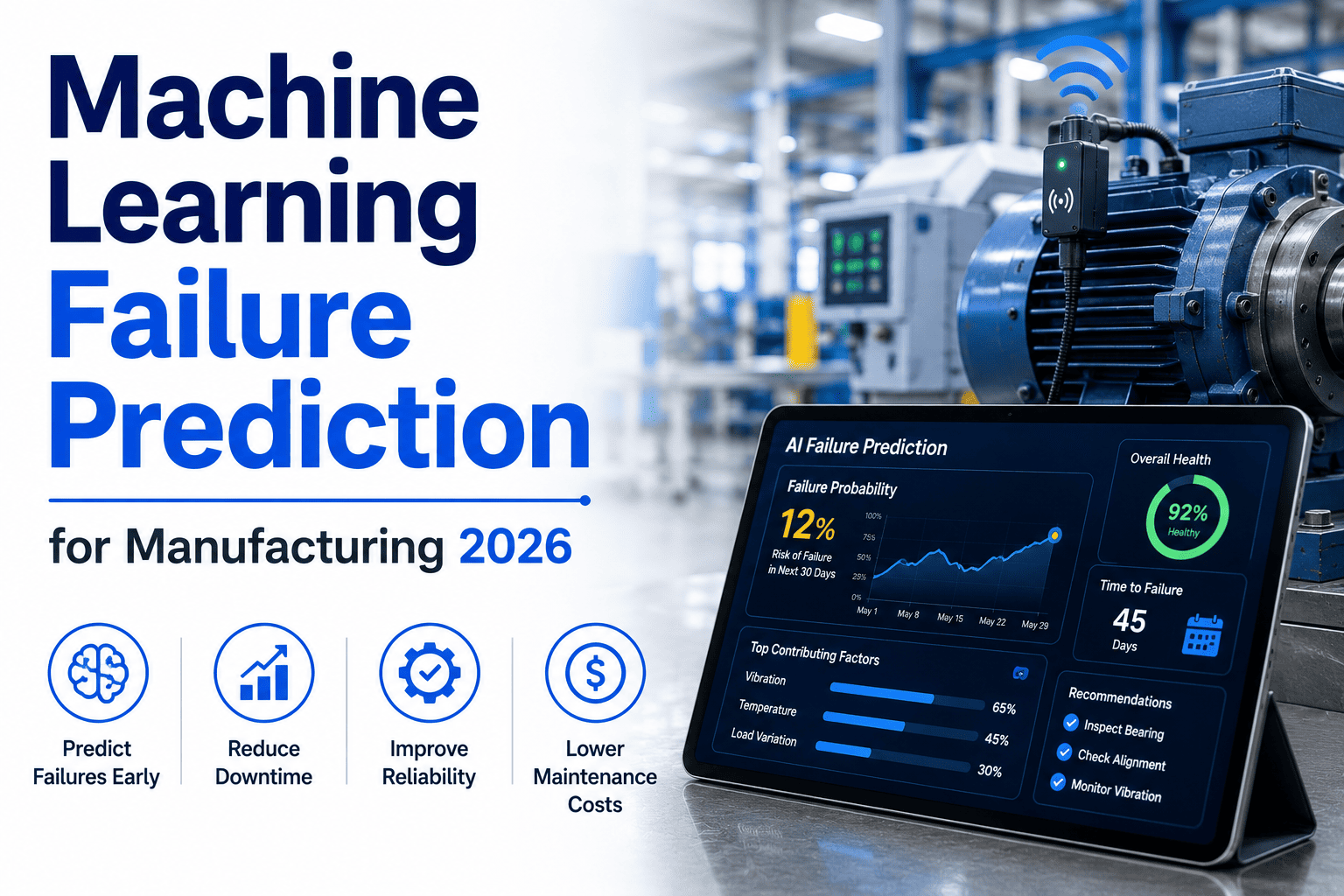
Manufacturing downtime now averages $260,000 per hour across heavy industry, and the gap between best-in-class plants (85% OEE) and the median (60%) is almost entirely a predictive-maintenance gap. Modern machine learning failure-prediction systems surface bearing, motor, and process-equipment faults 3–12 weeks before a human analyst would flag them — but only when the data pipeline, feature engineering, and CMMS integration are architected correctly. This 2026 guide breaks down how ML models are trained on vibration, current, and process signals, how anomaly scoring is tuned to suppress false positives, and how auto-generated work orders close the loop inside your CMMS. Ready to skip the theory? Start Free Trial and connect your first asset stream in under an hour.
Predictive Maintenance · 2026 Guide
What if your plant knew which asset would fail — 12 weeks before it did?
Machine-learning failure prediction shifts maintenance from reactive firefighting to planned intervention. Trained on vibration, current draw, temperature, and process telemetry, production-grade ML models now catch 80–92% of impending equipment failures with false-positive rates under 5%.
Median lead time ML models give maintenance teams before critical failure — versus 3–5 days for threshold-based alarms.
The Failure Window
Three signals machine learning reads that humans cannot
A single rolling-element bearing generates thousands of vibration samples per second. The degradation pattern that precedes a spall or race failure is measurable 20–60 days before it becomes audible — but only if the ML pipeline captures the right features at the right sample rate.
Vibration spectra (FFT + envelope)
Accelerometers at 25.6 kHz capture bearing defect frequencies (BPFO, BPFI, BSF). ML models trained on envelope spectra detect inner-race faults 3–8 weeks before ISO 10816 velocity thresholds trip. A 50 hp motor typically shifts from 1.2 mm/s RMS to 4.5 mm/s over 6 weeks; ML flags the trajectory at week one.
Motor current signature analysis (MCSA)
Current draw on a 3-phase induction motor encodes rotor bar, stator winding, and load-coupling health. A 2% harmonic shift at the pole-pass sideband frequency predicts rotor degradation 4–10 weeks out — invisible to a standard SCADA trend chart set at 5-second polling.
Process telemetry fusion
Temperature, pressure, flow, and run-speed deltas — when fused into a multivariate model — reveal drift that no single sensor catches. A heat exchanger fouling 0.3°C per week looks normal until the ML model compares it against 18 months of identical-load baselines and flags the divergence.
Feature Engineering
From raw sensor data to model-ready features
Feature engineering is where 70% of predictive-maintenance projects fail. A vibration waveform is not a feature — RMS, kurtosis, crest factor, and spectral band energy are. Below is the transformation pipeline that turns 25.6 kHz sensor streams into the 40–120 features a gradient-boosted model actually consumes.
Time-domain feature
RMS = √( Σxᵢ² / N )
Root-mean-square of vibration amplitude. Baseline for severity tracking; a 2× jump from baseline triggers investigation in most ISO 18436-2 programs.
Impulse feature
Crest = Peak / RMS
Crest factor rises early in bearing fatigue because impacts spike the peak before RMS moves. A crest factor above 6.0 on a healthy-bearing baseline (typically 3.5–4.5) is an early-warning flag.
Anomaly score
A(x) = Σ wᵢ · σ⁻¹(fᵢ)
Weighted sum of normalized feature deviations from the learned healthy-state distribution. Scores above 0.85 correspond to P(failure within 30 days) > 72% on validation sets.
| Sensor input | Sample rate | Engineered features | Model input count | Typical lead time |
|---|---|---|---|---|
| Triaxial accelerometer | 25.6 kHz | RMS, kurtosis, crest, FFT bands (8), envelope (6) | 18 per axis | 3–8 weeks |
| 3-phase current clamp | 10 kHz | MCSA sidebands, THD, imbalance, harmonics 1–7 | 14 | 4–10 weeks |
| RTD / thermocouple | 1 Hz | Delta-T, rate-of-change, load-normalized temp | 6 | 2–6 weeks |
| Process flow + pressure | 0.5 Hz | Efficiency ratio, fouling coefficient, drift slope | 9 | 4–12 weeks |
| Oil sensor (ferrous debris) | 0.1 Hz | Particle count trend, ferrous rate, viscosity index | 5 | 6–16 weeks |
Model Training & Tuning
The 6-month path from raw data to 90% recall
A production ML failure-prediction model is not a notebook experiment. It takes 4–6 months of disciplined iteration — baseline collection, supervised labelling, architecture selection, and false-positive suppression — to reach the 88–93% recall and <5% false-positive rate that maintenance teams will actually trust.
Baseline & data audit
Tag every critical asset, verify sensor health, backfill 12–18 months of historian data. Identify gaps — 60% of plants discover missing or mis-calibrated sensors at this stage. Output: clean multivariate time-series for 80%+ of in-scope assets.
Feature engineering + labeling
Build the feature library (RMS, kurtosis, spectral bands, MCSA sidebands). Label historical failures using CMMS work-order history — a 200-asset plant typically yields 40–80 labelled failure events across 12–18 months, enough for supervised learning.
Model selection & first training
Train XGBoost (tabular features), 1D-CNN (raw spectra), and Isolation Forest (unsupervised anomaly). Cross-validate on time-split folds. Most manufacturing teams land on XGBoost + Isolation Forest hybrid — best interpretability, lowest compute, 88–92% recall.
False-positive tuning
The hardest phase. Tune the anomaly threshold so false alarms stay under 5% — above that, technicians ignore the system. Use cost-sensitive learning: weight missed failures 10× higher than false alarms. Introduce a 2-of-3 confirmation rule across sensor modalities.
CMMS integration
Connect the model output to your CMMS (Maximo, SAP PM, Fiix, or UpKeep) via REST API. Each high-confidence alert auto-generates a work order with asset ID, predicted failure mode, recommended action, and due date — typically 7–14 days out.
Pilot validation & rollout
Run shadow mode for 30 days — model predicts, humans act as normal. Compare. A successful pilot shows 3+ true-positive catches and <2 false alarms per 50 assets per month. Then expand from pilot cell to full plant.
Worked Example
A 180-asset plant: from $42K/month in unplanned downtime to $6K
Consider a Midwest food-processing plant running 180 critical assets — mixers, conveyors, HVAC fans, ammonia compressors — with $42,000 average monthly unplanned-downtime cost and 14 hours MTTR. Here is what happens when ML failure prediction goes live across months 1–6.
$42K
Monthly downtime — baseline
$11K
Monthly downtime — month 4
$6K
Monthly downtime — month 6
3.2 hr
MTTR after planned interventions
86%
Failures caught with >14-day lead
4.1 mo
Payback period on ML platform + sensors
“
The model flagged a gearbox bearing on Line 4 six weeks before we would have caught it. We scheduled the swap during a sanitization window — zero lost production. That single catch paid for the entire annual platform license.
— Reliability Lead, 180-asset food-processing plant
Stop finding failures. Start predicting them.
Deploy ML failure prediction across your plant in under 30 days. Connect sensors, train models, and auto-generate CMMS work orders — no data science team required.
FAQ
Machine learning failure prediction — answered
How much historical data do we need before ML failure prediction works?
Most production models need 12–18 months of sensor historian data plus labelled failure events from your CMMS. With fewer than 8–10 labelled failures per asset class, unsupervised anomaly detection (Isolation Forest, autoencoder reconstruction error) is a better starting point than supervised classification — you can layer supervised models on once the failure log grows.
What false-positive rate can we realistically expect?
A well-tuned model on a mature data pipeline holds false positives under 5%. The lever is threshold calibration: cost-sensitive learning weights missed failures 10× higher than false alarms, and a 2-of-3 sensor-confirmation rule suppresses single-sensor noise. Above 8% false positives, technician trust collapses — tuning to that ceiling is non-negotiable. Book a Demo to see live false-positive dashboards.
Does the model work with our existing CMMS (Maximo, SAP PM, Fiix)?
Yes — integration is via REST API. When the ML model issues a high-confidence alert (anomaly score > 0.85), it auto-creates a work order with asset ID, predicted failure mode, recommended action, and a due date typically 7–14 days out. The work order flows through your normal approval queue, so planners retain control. No CMMS rip-and-replace required.
How is this different from our existing condition-monitoring thresholds?
Threshold alarms (ISO 10816 velocity limits, temperature caps) fire after the damage is already measurable — typically 3–5 days before failure. ML models read the trajectory and multivariate correlation, catching the same fault 3–12 weeks earlier. A bearing at 4.5 mm/s RMS has already spalled; ML flags the crest-factor drift at 1.4 mm/s, weeks earlier.
What does deployment cost and how fast is payback?
For a 150–250 asset plant, total cost (platform license + sensors + integration) runs $45K–$80K for year one. With typical unplanned-downtime savings of 60–75%, most plants reach payback in 4–7 months. A single caught catastrophic failure — a gearbox, compressor, or main drive — often covers the full annual cost. Start Free Trial to model the ROI on your asset list.
Your next failure is already in the data. Find it first.
Join the plants running 85%+ OEE on ML-powered predictive maintenance. Connect your first asset stream today — setup takes under an hour.
Free 14-day trial · No credit card