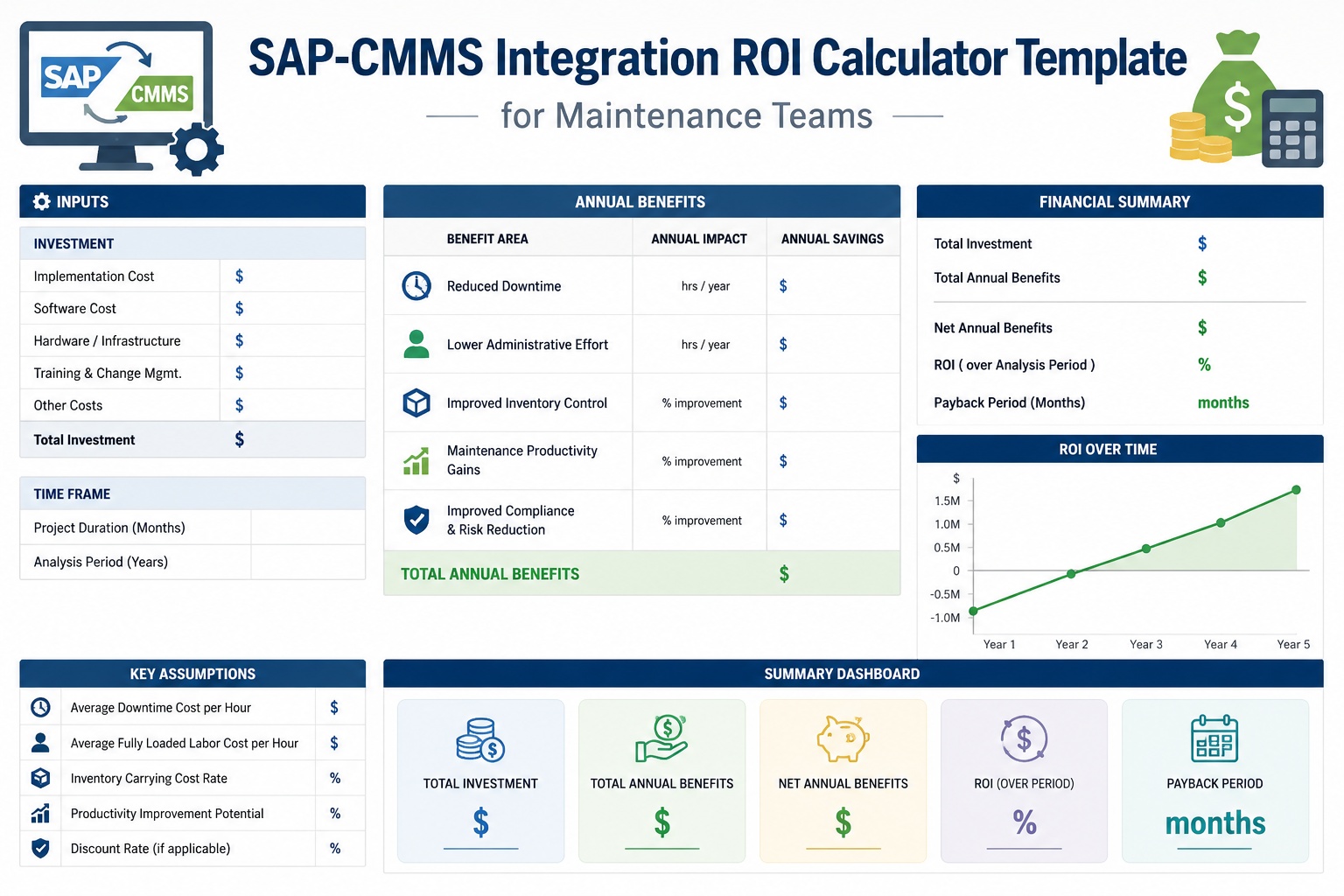
Maintenance executives can model the ROI of an SAP-CMMS integration to within 10-15% accuracy if they have the right inputs and a structured calculation framework. Most don't, because they're working from vendor marketing decks rather than from a disciplined model. The result is business cases that overstate savings, understate effort, and lose credibility with finance the first time they're stress-tested. This ROI calculator template provides the structured framework—inputs, calculation logic, and output—that survives finance scrutiny and produces a defensible investment case. Book a free demo to walk through the calculator on your numbers.
8
Operational input variables required for a defensible SAP-CMMS ROI model
Source: This calculator
5
Distinct savings categories that aggregate into total annual benefit
Source: This calculator
3-9 mo
Typical payback period for mid-complexity SAP-CMMS integrations with disciplined business case
Source: Industry benchmarks
±15%
Accuracy band achievable with structured calculator vs vendor-supplied estimates
Source: Business case research
Why ROI Models Determine Investment Approval
The single most important predictor of whether a SAP-CMMS integration gets approved isn't the technology, the vendor selection, or even the strategic case. It's the credibility of the financial model presented to the capital approval committee. A model that traces every dollar of claimed savings to a specific operational lever, supported by current-state inputs and conservative assumptions, survives stress-testing and gets approved. A model that aggregates vendor-supplied benefit percentages without showing the underlying math loses credibility on first review and gets sent back for rework—often killing the project's momentum entirely.
The discipline that distinguishes defensible business cases is structural transparency. Inputs are current-state operational measurements, not aspirational targets. Calculation logic is explicit and reproducible. Output metrics include both upside (best-case) and downside (worst-case) scenarios. Sensitivity analysis identifies the assumptions that matter most. Maintenance and finance leaders ready to operationalize this discipline on a current integration case can Sign up free to deploy the structured ROI calculator on a live business case.
The SAP-CMMS Integration ROI Calculator
The calculator below shows the eight operational inputs, five savings categories, and four output metrics that together produce a defensible annual ROI estimate. Sample values represent a typical mid-size industrial operation; replace each input with your own current-state measurement to produce a model specific to your context.
S1Downtime Reduction
25% reduction in unplanned downtime × hourly cost
I4 · I5
$3,000,000
S2PM Compliance Gain
Remaining unplanned events reduced 20% via better PM execution
I3 · I4 · I5
$1,800,000
S3Admin Productivity
30% reduction in maintenance admin hours from automation
I7 · I8
$585,000
S4Inventory Optimization
18% MRO reduction × 25% annual carrying cost
I6
$225,000
S5Energy Efficiency
5% reduction in energy spend via condition monitoring
I2
$500,000
Total Annual Savings
Sum of S1 through S5
All
$6,110,000
Software license / subscription
$300,000
Implementation services
$1,200,000
Internal team allocation
$400,000
Training & change management
$100,000
Total Year 1 Investment
$2,000,000
OUTPUT METRICS
ROI Summary
Total Annual Savings
$6.1M
Sum of 5 categories
Year 1 Investment
$2.0M
License + Implementation + Internal + Training
Year 1 ROI
205%
(Savings − Investment) / Investment
Payback Period
3.9 mo
Investment ÷ Monthly Savings
The model's structural discipline is that every output traces back to operational inputs through explicit calculation logic. Finance reviewers can interrogate any number in the output by drilling back through the calculation to the source input. That traceability is what produces credibility when the model goes to capital approval. Maintenance and finance leaders ready to populate this calculator with their own operational numbers can Sign up free to model the calculator against current operational baselines.
Where the Annual Savings Come From
Each savings category in the calculator represents a distinct operational lever with its own assumption basis, evidence requirements, and risk profile. Understanding each lever individually—not just the aggregate—is what allows the business case to survive finance stress-testing.
S1
Downtime Reduction
$3.0M / 49% of total
The largest single lever. Integrated CMMS reduces unplanned downtime through faster fault response, better parts availability, and proactive condition-based intervention. 25% reduction is typical for first-year improvement; mature programs achieve 40%+.
Evidence Required
Current downtime hours by equipment class; blended hourly cost calculated from lost production value plus restoration cost
S2
PM Compliance Gain
$1.8M / 29% of total
Better PM execution prevents the failures that would otherwise become unplanned events. Moving compliance from 60% to 90%+ typically reduces remaining unplanned failures by 20-30%. This savings stacks on top of S1.
Evidence Required
Current PM compliance rate from SAP PM history; correlation analysis between PM compliance and unplanned failure rate
S3
Admin Productivity
$585K / 10% of total
Maintenance admin work (work order creation, parts requisition, time entry, reporting) consumes 25-40% of admin FTE time. Integration automation reduces this by 30-40%. FTEs redeployed to higher-value reliability work or attrition.
Evidence Required
Current admin FTE count and burdened cost; time-study of admin tasks; targeted automation scope from integration design
S4
Inventory Optimization
$225K / 4% of total
Integrated MRO inventory reduces stock-outs, obsolescence, and duplicate ordering. 15-20% inventory reduction is typical; annual savings calculated from carrying cost (typically 22-28% of inventory value annually) rather than one-time release.
Evidence Required
Current MRO inventory value; annual carrying cost rate from finance; baseline obsolescence/write-off rate
S5
Energy Efficiency
$500K / 8% of total
Condition-monitored equipment runs at higher efficiency. Bearings replaced before they degrade, alignment maintained, lubrication optimized. 3-7% energy reduction on the monitored equipment population is typical for first-year benefit.
Evidence Required
Energy cost as a percentage of total maintenance spend; baseline efficiency by equipment class; condition monitoring scope
The relative contribution of each lever varies by industry and operational maturity. Industries with high downtime costs (refining, mining, power generation) skew heavily toward S1 and S2. Industries with large maintenance organizations skew toward S3. Capital-intensive operations with significant MRO inventory weight S4 more heavily. The calculator structure stays the same; the relative magnitude of each category adjusts based on which inputs dominate the specific operation. Business case authors ready to apply the lever framework to their industry context can Sign up free to model lever sensitivity for the current operating profile.
See the Calculator Running on Real Operational Numbers
Walk through the ROI calculator with actual maintenance data from a comparable operation, with input population, sensitivity analysis, and finance-ready output package. 30-minute live walkthrough.
Building a Defensible Business Case From the Calculator
The calculator output is the financial heart of the business case but isn't the business case itself. A defensible case wraps the calculator with the contextual narrative finance committees expect: current-state evidence, lever-by-lever rationale, conservative assumptions, risk-adjusted ranges, and explicit sensitivity to the assumptions that matter most.
Week 1
Input Population & Validation
Gather 8 operational inputs from current systems and operations leadership. Validate each input with the data owner. Document assumption basis for any value that requires estimation rather than measurement.
Weeks 2-3
Lever Stress-Testing
For each of the 5 savings categories, validate the assumption percentages against industry benchmarks and historical performance. Adjust for operational maturity. Build sensitivity scenarios (best/base/worst case).
Week 4
Investment Sizing & Risk Adjustment
Size Year 1 investment with vendor and implementation partner. Build risk-adjusted scenarios for cost overrun and schedule slippage. Document risk-mitigation assumptions in business case narrative.
Weeks 5-6
Finance Review & Committee Submission
Pre-review with CFO or finance partner. Address pre-review feedback. Finalize business case package. Submit to capital approval committee with executive summary, full model, and sensitivity analysis.
By week 6, the business case package is positioned for committee approval with three documents: the executive summary explaining the strategic and operational rationale, the calculator showing the savings derivation, and the sensitivity analysis showing how output metrics change under different assumption scenarios. That package addresses the questions finance committees actually ask rather than the questions vendors expect them to ask. Business case leads ready to build this package on a current opportunity can Book a free demo to build the business case package on a current opportunity.
Expert Perspective: What Distinguishes Approved Business Cases
The SAP-CMMS business cases I've seen approved cleanly share a property that often surprises new finance partners: they're more conservative than the vendor's model suggests. The savings percentages are at the low end of the industry range. The investment estimates include contingency. The payback periods are calculated against risk-adjusted savings rather than best-case savings. The cases that get sent back for rework almost always trace to one of three patterns—savings estimates without operational evidence to support them, investment estimates that look optimistically low to a CFO who has seen ERP implementations before, or sensitivity analysis missing entirely. The pattern that wins approval is patient, conservative, evidence-backed modeling. The pattern that loses is enthusiastic, vendor-supplied, narrative-light modeling. The capital committees know the difference.
Conservative Beats Optimistic
Savings percentages at the low end of industry range. Investment estimates with contingency. Payback against risk-adjusted savings. The CFO has seen ERP cases before; conservative modeling builds credibility.
Every Number Has Evidence
Each input traces to a current-state measurement. Each assumption traces to industry benchmark or historical performance. Numbers without traceable evidence get challenged and weaken the case.
Sensitivity Analysis Is Required
Capital committees expect to see how output changes under different assumption scenarios. Cases without sensitivity analysis appear naïve and get sent back for rework. Include three scenarios as standard practice.
Sensitivity Analysis: Stress-Testing the Model
The calculator output of $6.1M annual savings and 3.9-month payback represents the base case. Capital committees expect to see how those numbers change under best-case and worst-case scenarios. The table below shows the sensitivity bands typical for the five savings categories.
Swipe to compare scenarios
75%
Worst-case Year 1 ROI still positive — robust investment thesis
S1+S2
Levers carrying most upside & downside — highest sensitivity
The defensibility test for the model is what happens to the output if the worst-case assumptions apply. A model that produces positive ROI even in the worst-case scenario is a robust investment thesis. A model that requires base-case or better to produce positive ROI is fragile and gets pushback. The calculator above produces 75% Year 1 ROI even with worst-case assumptions, which positions it as a robust thesis for committee approval.
Build the Business Case That Actually Gets Approved
Eight operational inputs. Five savings levers. Three scenarios. Finance-ready output package. See the calculator running on real maintenance data with full sensitivity analysis.
Frequently Asked Questions
How do we determine the blended hourly downtime cost for input I5?
Blended downtime cost combines lost production value, restoration cost, and indirect impacts. The standard calculation: hourly contribution margin from lost production (revenue minus variable cost) plus average restoration cost per hour of downtime (parts, labor, expediting) plus indirect impact (customer impact, idle workforce). For a single production unit, this is straightforward. For multi-unit operations, weight by criticality—the downtime cost of the bottleneck unit is the operation's downtime cost. Many organizations underestimate this number; conservative estimates often run too low rather than too high.
What if our PM compliance baseline (I3) is already high (above 85%)?
A high PM compliance baseline means smaller S2 (PM Compliance Gain) savings but doesn't necessarily reduce total ROI. Operations with high baseline compliance often have other opportunities the calculator captures elsewhere—better MRO inventory optimization (S4), more administrative consolidation (S3), or larger energy efficiency upside (S5). Re-weight the calculator's expected percentages: lower S2 by 50%, but check whether S3 or S4 should be increased by 20-30% to reflect the operational maturity. The total often stays surprisingly similar.
How do we handle multi-site or multi-business-unit operations?
For multi-site operations, run the calculator once per site or business unit, then aggregate. Site-level inputs differ meaningfully (different equipment populations, different downtime costs, different MRO bases), so a single aggregate model loses important variation. The aggregate ROI is the sum of site-level outputs minus shared overhead (corporate-level licensing, central support team, etc.). For larger portfolios (10+ sites), consider running the calculator for a representative subset and extrapolating, but always validate the extrapolation against bottom-up site-level analysis for the top 3-5 sites by maintenance spend.
Should we include capital savings (extended equipment life) in the model?
Extended equipment life is real but typically excluded from year-by-year ROI calculations because the savings materialize over 5-15 year horizons. Most finance committees prefer to see operational savings (S1-S5) with explicit annual realization, then treat extended equipment life as a separate strategic benefit not modeled in the financial case. If equipment-life extension is included, model it as a depreciation savings (deferred capital investment) rather than as a cash savings, and include only the portion expected to materialize within the financial planning horizon (typically 3-5 years).
What sensitivity ranges should we use for finance review?
The sensitivity ranges in the table above are typical for mid-complexity integrations. Worst case typically uses 50-60% of base-case assumptions; best case uses 130-160%. Higher uncertainty (newer technology, less benchmark data) warrants wider ranges (40-180%); lower uncertainty warrants tighter ranges (70-130%). The ranges should be defensible against industry benchmarks, not arbitrary. Finance committees often ask "what would have to be true for the worst case to materialize," so document the explicit assumptions that drive each scenario rather than just presenting numbers.