Commercial buildings account for nearly 40% of global energy consumption, yet most facility managers still operate on fixed setpoints, manual scheduling, and reactive utility bill reviews. AI-driven energy optimisation changes the operating model: instead of reacting to last month's utility invoice, the platform continuously monitors HVAC loads, lighting zones, BMS setpoints, and occupancy patterns to trim 20 to 40% from energy spend without capital replacement. This guide covers the AI optimisation strategies, technology stack, and implementation sequence that deliver measurable results within the first 90 days. Sign up free on Oxmaint to begin tracking your building energy data, or book a demo for an energy optimisation walkthrough for your portfolio.
Start Reducing Your Building Energy Costs With AI Today
Oxmaint's energy and sustainability module tracks HVAC, lighting, and utility data across your portfolio and surfaces optimisation opportunities automatically. Live in 14 days, no infrastructure replacement required.
Energy Optimisation in Commercial Buildings: Key Numbers
40%
Share of global energy consumed by commercial and residential buildings, making facilities the single largest addressable energy reduction opportunity for sustainability programmes
30%
Average commercial building energy waste from poor scheduling, oversized setpoints, and unoccupied space conditioning — all addressable through AI-driven optimisation without equipment replacement
$0.30
Average energy cost per square foot per year in US commercial office buildings, representing the second-largest operating expense after labour and the most controllable line item in any FM budget
18mo
Typical payback period for AI energy optimisation platform investment including hardware, software, and implementation across a 10-building commercial portfolio at current utility rates
What AI Energy Optimisation Actually Does
AI energy optimisation continuously analyses building occupancy patterns, weather data, equipment load curves, and utility rate schedules to adjust HVAC setpoints, lighting levels, and equipment run schedules in real time. Unlike static building automation programming, AI adapts as occupancy patterns change, as weather varies, and as equipment ages. The result is consistent 20 to 40% energy reduction without comfort complaints or equipment stress.
HVAC Optimisation: 40 to 60% of Total Building Energy
HVAC systems consume 40 to 60% of commercial building energy in most climates. The gap between typical and optimal HVAC operation is large because most buildings run on commissioning-era schedules that no longer match actual occupancy, equipment that has drifted from optimal performance, and setpoints set conservatively to avoid complaints rather than to minimise energy use.
CO2-sensor-driven OA damper control reduces outdoor air conditioning load by 25 to 45% in variable-occupancy spaces. Conference rooms, lobbies, and open-plan floors with DCV save more energy per square foot than any other single HVAC measure.
Savings: 25 to 45% OA load
AI continuously adjusts supply air temperature, chilled water setpoints, and AHU static pressure based on zone demand, weather forecast, and occupancy schedule. Buildings with AI setpoint control use 15 to 22% less HVAC energy than those on fixed schedules.
Savings: 15 to 22% HVAC energy
Chiller sequencing, cooling tower fan speed control, and condenser water temperature reset based on wet bulb conditions reduce chiller plant energy by 18 to 30%. A chiller plant running 2 degrees warmer chilled water saves 4% energy per degree at equivalent cooling load.
Savings: 18 to 30% chiller plant
AI pre-cools buildings during off-peak rate periods using thermal mass, reducing demand charges during peak rate windows. For buildings on time-of-use tariffs, predictive pre-cooling reduces peak demand by 15 to 25% without adding energy consumption.
Demand savings: 15 to 25%
Lighting and Building Envelope: Secondary Energy Opportunities
| Measure | Energy Saving | Implementation | Payback Period |
| Occupancy-based lighting control |
30 to 50% lighting energy |
Occupancy sensors integrated with BMS; AI adjusts daylight harvesting based on weather and time |
1.5 to 3 years |
| Daylight harvesting zones |
20 to 35% perimeter lighting |
Photocell sensors with dimming ballasts; AI manages transition between daylight and artificial light |
2 to 4 years |
| LED retrofit plus smart control |
50 to 75% total lighting |
LED fixtures plus network control; AI-managed scenes and schedules reduce runtime hours |
3 to 5 years |
| Window management (smart glass) |
10 to 20% cooling load |
Electrochromic glass tint controlled by AI based on solar angle, occupancy, and cooling load |
7 to 12 years |
| Building envelope air tightness audit |
5 to 15% HVAC infiltration load |
Blower door test identifies infiltration paths; targeted sealing reduces conditioning load |
Under 1 year for sealing |
BMS Integration and AI Control Architecture
AI energy optimisation sits above the BMS control layer, sending adjusted setpoints to existing BMS equipment rather than replacing it. This integration approach means buildings with Siemens, Schneider, Johnson Controls, or Honeywell BMS can deploy AI optimisation without replacing existing hardware.
L1
Sensor and Metering Layer
Sub-meters, occupancy sensors, CO2 detectors, and smart thermostats feed real-time data to the AI platform. For buildings without sub-metering, clamp-on current sensors on panel feeders provide circuit-level energy data without panel work. The sensor layer is the foundation — AI accuracy scales directly with sensor coverage.
L2
BMS Integration Layer
BACnet IP, Modbus TCP, or REST API integration connects the AI platform to existing BMS. The integration layer reads current setpoints, occupancy schedules, and equipment status, then writes optimised setpoints back to the BMS at configurable intervals. No BMS replacement required for this layer.
L3
AI Optimisation Engine
Machine learning models analyse occupancy patterns, weather forecasts, utility rate schedules, and equipment performance data to calculate optimal setpoints for each zone and system. Models are trained on building-specific data during the first 30 days and improve continuously as the dataset grows.
L4
CMMS Integration Layer
Energy anomalies that indicate equipment degradation generate CMMS work orders automatically. A chiller running 15% above expected kW/ton triggers a predictive maintenance work order before efficiency loss becomes a comfort complaint. The CMMS layer is what connects energy waste to maintenance action.
Energy Analytics: Turning Utility Data Into Decisions
Energy Use Intensity (kBtu per square foot per year) normalises energy consumption across buildings of different sizes and types. Class A office EUI benchmarks at 65 to 80 kBtu/sq ft/year; buildings above 100 kBtu/sq ft/year have significant optimisation headroom. EUI tracking in Oxmaint compares each building against ENERGY STAR baselines for its specific use type and climate zone.
Demand charges often represent 30 to 50% of commercial electricity bills in the US but are driven by peak usage in a single 15-minute window per month. AI-managed load shedding, pre-cooling, and equipment sequencing during utility peak windows reduce demand charges without occupant impact. A 10% reduction in peak demand typically reduces electricity bills by 3 to 7% depending on tariff structure.
Automated fault detection algorithms identify equipment faults that waste energy but do not cause comfort complaints: economiser faults with simultaneous heating and cooling, AHU dampers stuck open, chiller condenser tube fouling, and air handler supply fan running above design static. Each fault type has a quantifiable energy waste signature that AI models detect weeks before manual identification.
AI analysis of 12 months of interval meter data identifies whether time-of-use, demand-based, or real-time pricing tariffs would reduce costs for each building's load profile. Tariff switching analysis in Oxmaint quantifies the annual saving from tariff changes before any operational changes are made, providing low-risk energy cost reduction through procurement rather than infrastructure investment.
ROI Framework: Building the Energy Optimisation Investment Case
Class A Office Tower (500,000 sq ft)
AI HVAC and lighting optimisation
$180K to $380K
Annual energy cost reduction from AI setpoint optimisation, DCV deployment, and demand charge management. Based on $0.30/sq ft baseline and 25% average reduction across HVAC and lighting systems.
Baseline: $150,000 annual energy at $0.30/sq ft; 18-month payback on platform investment
Multi-Site Portfolio (10 buildings, 2M sq ft)
Portfolio-wide AI energy programme
$720K to $1.8M
Annual savings across a 10-building commercial portfolio with consistent AI optimisation deployment. Portfolio-level demand charge management and cross-building load shifting add 8 to 12% additional saving above single-building deployments.
Payback: 12 to 18 months including platform, sensors, and integration costs
ENERGY STAR Score Improvement
ENERGY STAR certification impact
+$0.80/sq ft
Average rental premium commanded by ENERGY STAR certified commercial office buildings versus non-certified comparable buildings in the same market. For a 200,000 sq ft building, certification adds $160,000 to annual rental income in addition to energy cost savings.
ENERGY STAR requires score of 75+; AI optimisation typically drives 10 to 25 point score improvements
Carbon Credit Value
LEED, BREEAM, and voluntary carbon markets
$15 to $85/tonne
Carbon credit value range for verified building energy reduction projects in voluntary and compliance markets in 2026. A 500,000 sq ft office reducing energy by 25% generates approximately 1,200 to 1,800 tonnes of CO2 reduction annually for credit generation.
Additional revenue stream on top of direct energy cost savings for ESG-reporting portfolios
90-Day AI Energy Optimisation Implementation Sequence
01
Energy Audit and Baseline Establishment (Days 1 to 30)
Collect 12 months of interval meter data per building. Map sub-metering coverage and identify gaps. Conduct BMS point inventory to confirm integration protocol (BACnet, Modbus, or API). Calculate current EUI per building and benchmark against ENERGY STAR targets. Identify the top 5 energy waste sources per building from consumption pattern analysis.
Output: EUI baseline, BMS integration map, top-5 waste sources per building
02
Sensor and Integration Deployment (Days 15 to 45)
Install sub-meters, CO2 sensors, and occupancy sensors where coverage gaps exist. Configure BMS integration to pass setpoint control to the AI platform. Connect utility interval data feeds for demand charge monitoring. Commission Oxmaint energy module and verify data flow from all sensors and BMS points. First optimisation decisions are typically generated within 7 days of data connection.
Output: Full sensor coverage, live BMS integration, AI model training commenced
03
AI Model Training and Conservative Optimisation (Days 30 to 60)
AI models train on building occupancy patterns, weather response, and equipment load curves. Optimisation begins conservatively within comfort boundaries; setpoint adjustments limited to plus or minus 1 degree Celsius while baseline data accumulates. Demand charge alerts and anomaly detection active from day one. First energy saving results typically visible on the 30-day consumption comparison.
Output: 5 to 15% energy reduction in first 60 days from anomaly elimination alone
04
Full Optimisation and Performance Verification (Days 60 to 90)
Expand setpoint optimisation range as confidence intervals tighten. Activate predictive pre-cooling, demand charge management, and tariff optimisation. Generate 90-day energy report comparing kWh, demand charges, and EUI against pre-deployment baseline. Identify next optimisation opportunities from fault detection findings. Present board-ready energy performance report with verified savings.
Output: 20 to 40% energy reduction verified; board-ready performance report
Frequently Asked Questions: AI Energy Optimisation
QDoes AI energy optimisation require replacing existing BMS hardware?
No. AI platforms integrate with existing Siemens, Schneider, Johnson Controls, and Honeywell BMS systems via BACnet or Modbus without hardware replacement.
Sign up free to see the integration checklist, or
book a demo.
QHow quickly does AI energy optimisation produce measurable results?
Fault detection and anomaly elimination typically produce 5 to 15% savings within the first 30 days. Full AI optimisation results of 20 to 40% are usually verified at the 90-day mark.
Book a demo to model expected savings for your portfolio.
QWhat utility data is required to start an AI energy optimisation programme?
Minimum 12 months of interval meter data (15-minute readings) per building. Utility providers supply this via green button or API download.
Sign up free to connect your utility data to Oxmaint.
QCan AI energy optimisation data be used for ESG reporting and ENERGY STAR certification?
Yes. Oxmaint's energy module outputs are formatted for ENERGY STAR Portfolio Manager, GRI 302 energy disclosure, and GRESB reporting.
Book a demo to see the ESG reporting integration.
Reduce Your Commercial Building Energy Costs 20 to 40% With Oxmaint
AI setpoint optimisation, demand charge management, fault detection, and ENERGY STAR reporting across your full portfolio. Live in 14 days, no BMS replacement required.
AI Setpoint ControlDemand Charge ManagementFault DetectionENERGY STAR Reporting
Continue Reading: Energy and Sustainability